Study of Assembly Line Scheduling, an Application of Dynamic Programming

(1)

INTRODUCTION

Many decision-making problems involve a process that takes in several stages (multistage process) in such a way that at each stage, the process is dependent on the strategy choosen. Such type of problems are called Dynamic Programming Problems (D.P.P). Thus it is concerned with the theory of multistage decision process, i.e the process in which a sequence of interrelated decisions has to be made. A D.P.P is a decision-making problem in n-variables, the problem being sub-divided into n-subproblems each sub-problem being a decision-making problem in one variable only. The solution to a D.P.P is achieved sequencially starting from one stage to the next till the final stage is reached.

The concept of D.P.P is largely based upon the principle of optimality. “An optimal policy has the property that what ever the initial state and initial decisions are, the remaining decisions must constitute an optimal policy with regard to the state resulting from the first decision”². D.P.P is a

Study of assembly line scheduling,

An application of dynamic programming

SANJUKTA MOHANTY and PRAFULLA K. BEHERA

Department of Computer Science and Applications North Orissa University Sriramchandra Vihar, Takatpur Baripada, Mayurbhanj (India).

Department of Computer Science and Application Utkal University, Vani Vihar Bhubaneswar - 751 004 (India).

(Received: November 07, 2010; Accepted: September December 11, 2010)

ABSTRACT

This papers describes the design and implementation of an optimized base scheduling algorithm for multiple assembly lines (i = 1,2,…..,n) to solve manufactureing problems in a factory. The scheduling goal is to delivery products just in time in case of rush order comes in and when the customer wants the product to be manufactured as quickly as possible. If the demand of the product is high, then to increase the production rate in few time, the multiple assembly line scheduling technique can be applied.

Keywords: Dynamic programming, Assembly line, Scheduling, Optimization.

mathematical technique dealing with the optimization of multistage decision process. In D.P.P the optimum solution is obtained in an orderly manner.

(2)

if there are n machines each of which can perform m different kinds of work. Then question arises that if k jobs are to be performed what policy should be adopted for producing products in such a way that the total value of the products produced is maximized and also products should be produced in time.

If the dynamic programming problem is solved by using the recursive equation starting from the first through the last stage, i.e obtaining the sequence f₁→ f₂→ f₃→ …… → f_N the computation involved is called the forward computational procedure. If the recursive equation is formulated

in a different way so as to obtain the sequence f_N

→ f_N-1→ _……→ f₁. Then the computation is known

as the backward computational procedure2,3_.

Dynamic programming algorithm can be broken into a sequence of four steps. That are

´ Characterize the structure of an optimal

solution.

´ Recursively define the value of an optimal

solution.

´ Compute the value of an optimal solution in

a bottom-up fashion.

´ Construct an optimal solution from computed

information.

Dynamic programming can design and implement an optimized- base scheduling algorithm for multiple assembly lines i (i = 1,2…m). It solves manufacturing problems to find the fastest way through a factory using multiple assembly lines. The increasing market demand for product variety forces the manufacturer to design multilevel assembly lines for which products can be manufactured as quickly as possible. If occasionally a rush order comes in and costomer wants the product to be manufactured as quickly as possible, then this problem can easily

be solved using multilevel assembly line scheduling1_.

Basic concept of assembly-line scheduling

In manufacturing systems, the assembly line has become one of the most valuable researches to accomplish the real world problems related to them. A manufacturing system could be defined as a collection of integrated equipment (including production machines and tools, material handling and work-positioning devices and

computer systems) and human resources, whose function is to perform one or more processing and/ or assembly operations on raw material, a part, or set of parts. In this study, the discussion will focus

on assembly line system6_.

In a manufactureing company manufacturing problems can be solved using assembly line scheduling. Assembly line scheduling design consists of one or more assembly lines, with more than one workstations in each assembly line. Each assembly line contains equal number of stations. The functions of stations in a assembly line are different. But the working functions of stations in a assembly line is same as the working functions of corresponding stations of other assembly lines. For example the jth station on assembly line 1 performs the same function as jth station on other assembly lines. The stations are built in different times and with different technologies.

Characteristics of assembly lines

An assembly line consists of a sequence of tasks, each having an operational processing time and a set of precedence relations, is widely adopted

in manufacturing plans7_{. There is a work element}

and workstations as a part in assembly lines. Then, it is better to know about a element and workstation first, before knowing all about the assembly lines. A work element is the smallest unit productive work that adds values to the product, such as tightening (thinning/reduction) a screw, welding, inserting a gear assembly. A workstation is also dubbed as a collection of a set of work elements that are performed there. A product is passed down the line and visits each workstation in sequence. An assembly line contains of a set of sequential workstations, typically connected by a continuous material handling system. It is designed to assemble component parts of a product and perform any related operations to produce the finished product. There also other components in there, namely workers (manual and robotics), a material handling system (conveyors), buffers, unloading and storage

space, layout (linear, u-shape and others)4_.

Also few definations of assembly lines are

given by few researchers. Baker and Scholl8_said

(3)

J 1 2 3 4 5 6

a_1,j 7 9 3 4 8 2

a_2,j 3 5 6 4 2 3

a_3,j 2 3 5 4 7 6

l_i[j]

l₁[j] 2 3 1 1 2

l₂[j] 2 3 2 2 2

l₃[j] 3 3 3 3 3

f* ₂₈

l* ₁

f_i[j]

f₁[j] 9 17 13 17 25 26

f₂[j] 7 12 17 21 23 26

f₂[j] 5 8 13 17 24 30

J: 1 2 3 4 5

T1

2,j 1 2 4 5 1

T1

3,j 7 2 4 1 2

T2

1,j 2 1 5 6 3

T2

3,j 4 3 6 5 2

T3

1,j 3 1 4 2 5

T3

2,j 4 2 1 5 3

i: 1 2 3

e_i 2 4 3

x_i 1 3 4

means of mass and large scale productions. They are also dubbed as flow-oriented production systems which are still typical in the industrial production of high-quantity standardized commodities and even gain importance in

low-volume production of customized products. Lusa9

said that assembly lines could be defined as a production system made up of a ser ies of workstations that are connected by a conveyor belt or a similar system that transports the object that

is being assembled. Yaman10_{stated that assembly}

lines are an example of flow lines which is the most commonly used system in a mass-production

environment. Assembly lines enable the assembly of complex products by workers who have received

a short training period11_{. Thus, an efficient assembly}

line design, as a part of a manufacturing system, is a vital problem for some companies. An assembly line is a usual solution for medium and high-production volumes.

Design of assembly-line scheduling problem

Manufacturing problems can be solved using assembly line scheduling techniques. For example, Motor corporations produce automobiles in a factory that have multiple assembly lines. Each assembly line has n working stations, numbered j = 1,2,…..,n. When a lot enters an assembly line, it passes through that line only. Occasionally a special rush order comes in, and customer wants the product to be manufactured as quickly as possible. For rush orders the lot still passes through the n stations in order, but the factory manager may switch the partially-completed product from one assembly line to other after any station. The efficiency of jth station on line i is not equal with the jth stations on other assembly lines. The jth stations on assembly lines are made up of different technologies.

The objective of this paper is to develop a recursive algorithm to determine the fastest way through the factory, in case of rush order. We have to determine which station to choose from line 1, which station to choose from line 2,………., which station to choose from line m in order to minimize the total time through the factory for one product. Also if the demand of the product is high, then to increase the production rate in few time the lot changes an assembly line.

Notations used in the proposed recursive algorithm

(4)

(We have mentioned only S_1,j, S_m,j and T1 m,j, T

2

1,j, where j = 1 to n, but not all the stations Si,j and Ti,j, because diagram will be

much more complex)

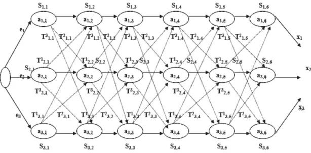
Fig. 1: Assembly line scheduling with ‘m’ assembly lines and ‘n’ stations

Fig. 2: Assembly line scheduling with 3 assembly lines and 6 work stations

balanced. An automobile chassis (in this paper we have taken the product as an automobile in motor corporation) enters each assembly line has parts added to it at a number of stations and a finished auto exits at the end of the line.

The following notations are used in our algorithm.

´ i - This is the assembly line, i = 1,2,...,m.

´ n - Each assembly line has n stations, where

n>1 and numbered j = 1,2,...,n.

´ S_i,j- This is denoted as jth station on line i,

(5)

For example:

S_1,j- This is jth station on line 1. S_2,j- This is jth station on line 2.

´ a_i,j- This is the assembly time required at

station S_i,j.

´ e_i- This is the entry time for the chassis to

enter assembly line i.

´ x_i- This is an exit time for completed auto to

exit assembly line i.

´ T1

i,j - This is the time to transfer a chassis

away from assembly line i after having gone

through the station S_i,j, where i =

2,3,……….,m and j = 1,2,……….,n-1 to the

respective stations S_i,j, where i = 1 and j =

2,3,……….,nof assembly line 1.

That is for i = 2 and j = 1,2,……….,n-1

T1 2,1,T

1

2,2,……….,T

1

2,n-1 - These are the

times required to transfer a chassis away from assembly line 2 after having gone through the stations S_2,1,S_2,2,……….,S_2,n-1 of assembly line 2 to

assembly line 1 of stations S_1,2,S_1,3,……….,S_1,n

respectively.

For i = 3 and j = 1,2,……….,n-1

T1 3,1,T

1

3,2,……….,T

1

respectively.

………...

For i = m and j = 1,2,……….,n-1

T1 m,1,T

1

m,2,……….,T

1

m,n-1 - These are the

times required to transfer a chassis away from assembly line m after having gone through the

stations S_m,1,S_m,2,……….,S_m,n-1 of assembly line m

to assembly line 1 of stations S_1,2,S_1,3,……….,S_1,n

respectively.

T2

i,j- This is the time to transfer a chassis

away from assembly line i after having gone through

the station S_i,j, where i = 1,3,4,……….,m and j =

1,2,……….,n-1 to the respective stations S_i,j, where

i = 2 and j = 2,3,……….,nof assembly line 2.

T2 1,1,T

2

1,2,……….,T

2

respectively.

For i = 3 and j = 1,2,……….,n-1

T2 3,1,T

2

3,2,……….,T

2

respectively.

………...

(6)

………...

For i = m and j = 1,2,……….,n-1

T2 m,1,T

2

m,2,……….,T

2

respectively.

T3

i,j- This is the time to transfer a chassis

the station S_i,j, where i = 1,2,4,5,……….,m and j =

i = 3 and j = 2,3,……….,nof assembly line 3.

T3 1,1,T

3

1,2,……….,T

3

assembly line 3of stations S_3,2,S_3,3,……….,S_3,n

respectively.

For i = 2 and j = 1,2,……….,n-1

T3 2,1,T

3

2,2,……….,T

3

respectively. ……… ………... ……… ………...

For i = m and j = 1,2,……….,n-1

T3 m,1,T

3

m,2,……….,T

3

respectively.

………... ………...

Tm

i,j - This is the time to transfer a chassis

the station S_i,j, where i = 1,2,3,……….,m-1 and j =

i = m and j = 2,3,……….,nof assembly line m.

Tm 1,1,T

m

1,2,……….,T

m

assembly line m of stations S_m,2,S_m,3,……….,S_m,n

respectively.

For i = 2 and j = 1,2,……….,n-1

Tm 2,1,T

m

2,2,……….,T

m

respectively.

………... ………... For i = m-1 and j = 1,2,……….,n-1:

Tm m-1,1,T

m

m-1,2,……….,T m

m-1,n-1 - These are the times

required to transfer a chassis away from assembly

line m-1 after having gone through the stations S

m-1,1,Sm-1,2,……….,Sm-1,n-1 of assembly line m-1 to

respectively.

´ f_i[j] - This is the fastest possible time to get a

chassis from the starting point through

station S_i,j. This gives the value of optimal

solution to subproblem.

´ l_i[j] - This is the line number, 1 or 2 or……….or

m, whose station j-1 is used in a fastest way

through station S_i,j where i = 1,2,……….,m

and j = 2,3,……….,n. We have not defined

here l_i[1] because no station precedes station

on the lines i = 1,2,……….,m.

´ f* _{- This is the fastest time to get a chassis all}

the way through the factory.

´ l* _{- This is the line whose station n is used in}

a fastest way through the entire factory.

MATERIAL AND METHODS

(7)

The fastest way of the auto can be

considered through station S_1,j or S_2,j or ……….or

S_m,j where j=1,2,……….,n.

´ If the fastest way of the auto will be

considered through station S_1,j, then it must go

through station j-1 on lines 1,2 or 3,...,or m. So

there are m_c

1 choices for the fastest way through

station S_1,j. That is,

´ The fastest way through station S_1,j-1 and

then directly through station S_1,j. The time for going

from station j-1 to station j on the same line being negligible.

Or

The fastest way through station S_2,j-1, a

transfer from line 2 to line 1, then through station S_1,j. The transfer time being T1

2,j-1.

...

………... Or

In this way the last choice is that, the auto

chassis could have come from station S_m,j-1 and then

been trasfered to station S_1,j, the transfer time being T1

m,j-1.

Therefore there are m_c

1 choices for the fastest way

through station S_1,j. So in this case the chassis must

go through station j-1 on lines 1 or 2 or 3 or………or m.

´ If the fastest way of the auto will be

considered through station S_2,j, then it must go

through station j-1 on lines 1,2 or 3,...,or m. So

there are m_c

1 choices for the fastest way through

station S_2,j.

That is,

The fastest way through station S_2,j-1 and

then directly through station S_2,j. The time for going

from station j-1 to station j on the same line being negligible.

Or

The fastest way through station S_1,j-1, a

transfer from line 1 to line 2, then through station

S_2,j. The transfer time being T2

1,j-1. ……………………………………………………………………………………………………………………………………………………

Or

In this way the last choice is that, the auto

chassis could have come from station S_m,j-1 and then

been trasfered to station S_2,j, the transfer time being T2

m,j-1.

Therefore there are m_c

1 choices for the

fastest way through station S_2,j. So in this case the

chassis must go through station j-1 on lines 1 or 2 or 3 or………or m.

……… In this way there are m_c

1 choices for the fastest way

through each stations S_1,j,S_2,j,……….,S_m,j. Therefore

the total number of choices through stations S_i,j is

m * m_c

1 = m * m = m 2_.

A recursive solution

In dynamic programming paradism the value of an optimal solution is defined recursively in terms of the optimal solutions to subproblems. Here the subproblems are considered as to find the fastest way through station j on the lines i = 1,2,……….,m for j = 1,2,……….,n.

Let f_i[j] denote the fastest possible time to get a chassis from starting point through station S_i,j.

Here also we have to determine the fastest time to get a chassis all the way through the factory

which is denoted by f*_{. The chassis has to get all}

the way through station n on lines 1 or 2 or……….or m and then to the factory exit. Since the faster of these ways is the fastest way through the entire factory, we have

f*_{= min ( f}

1[n] + x1, f2[n] + x2,……….,fm[n] + xm ).

To get the fastest way through station 1 on lines i = 1,2,……….,m a chassis just goes directly to that station. Thus we have

f₁[1] = e₁ + a_1,1 f₂[1] = e₂ + a_2,1

………... ………... f_m[1] = e_m + a_m,1

Now to compute f_i[j] for j = 2,3,……….,n we have

m_c

1 choices discussed in the section 5. From

m_c 1

choices, using 1st_{choice we have,}

f₁[j] = f₁[j-1] + a_1,j and in the latter cases we have , f₁[j] = f₂[j-1] + T1

2,j-1 + a1,j

……….…….….………….……….. f₁[j] = f_m[j-1] + T1

m,j-1 + a1,j

(8)

f₁[j] = e₁ + a_1,1, if j = 1.

= min ( f₁[j-1] + a_1,j, f₂[j-1] + T1

2,j-1 + a1,j,……….,

f_m[j-1] + T1

m,j-1 + a1,j ), if j >= 2.

f₂[j] = e₂ + a_2,1,if j = 1.

= min ( f₂[j-1] + a_2,j, f₁[j-1] + T2

1,j-1 + a2,j,……….,

f_m[j-1] + T2

m,j-1 + a2,j ), if j >= 2.

……….…….….……….….. f_m[j] = e_m + a_m,1,if j = 1.

= min ( f_m[j-1] + a_m,j, f₁[j-1] + Tm

1,j-1 + am,j, f2[j-1] +

Tm

2,j-1 + am,j,………., fm-1[j-1] + T m

m-1,j-1 + am,j ), if j

>= 2.

Now we consider l_i[j] be the line number 1 or 2

or……….or m whose station j-1 is used in a fastest

way through station S_i,j for i = 1,2,……….,m and j =

2,3,……….,n.

Let l*_{be the line whose station n is used in a fastest}

way through the entire factory.

Counting the fastest times

The f_i[j] values give the optimal solutions

to subproblems. f_i[j] depends on the values of f₁

[j-1], f₂[j-1],……….,f_m[j-1]. The fastest way the factory

can be computed by computing the f_i[j] values in

order of increasing station numbers j = 1,2,……….,n.

Proposed algorithm-1

1. For k = 1 to n, f_k[1] = e_k + a_k,1

2. For j = 2 to n,

3. Do if f₁[j-1] + a_1,j <= f₂[j-1] + T1

2,j-1 + a1,j && f3

[j-1] + T1

3,j-1 + a1,j && ……….&& fm[j-1] + T 1

m,j-1 +

a_1,j

4. Then f₁[j] = f₁[j-1] + a_1,j

5. l₁[j] = 1

6. Else if f₂[j-1] + T1

2,j-1 + a1,j <= f1[j-1] + a1,j &&

f₃[j-1] + T1

3,j-1 + a1,j &&……….&& fm[j-1] + T 1

m,j-1 + a1,j

7. Then f₁[j] = f₂[j-1] + T1 2,j-1 + a1,j

8. l₁[j] = 2

9. Else if f₃[j-1] + T1

3,j-1 + a1,j <= f1[j-1] + a1,j &&

f₂[j-1] + T1

2,j-1 + a1,j &&……….&& fm[j-1] + T 1

m,j-1 + a1,j

10. Then f₁[j] = f₃[j-1] + T1 3,j-1 + a1,j

11. l₁[j] = 3 // m_c

1 number of conditions have been

checked to compute f_i[j] for i = 1 and j>=2

(lines 3 to 12) ……….………

12. Else if f_m[j-1] + T1

m,j-1 + a1,j <= f1[j-1] + a1,j &&

f₂[j-1] + T1

2,j-1 + a1,j &&……….&& fm-1[j-1] + T 1

m-1,j-1 + a1,j

13. Then f₁[j] = f_m[j-1] + T1 m,j-1 + a1,j

14. l₁[j] = m

15. If f₂[j-1] + a_2,j <= f₁[j-1] + T2

1,j-1 + a2,j && f3[j-1]

+ T2

3,j-1 + a2,j && f4[j-1] + T 2

4,j-1 + a2,j &&

……….&& f_m[j-1] + T2

m,j-1 + a2,j // To compute

f_i[j] for i = 2 and j >=2 16. Then f₂[j] = f₂[j-1] + a_2,j 17. l₂[j] = 2

18. Else if f₁[j-1] + T2

1,j-1 + a2,j <= f2[j-1] + a2,j &&

f₃[j-1] + T2

3,j-1 + a2,j &&……….&& fm[j-1] + T 2

m,j-1 + a2,j

19. Then f₂[j] = f₁[j-1] + T2 1,j-1 + a2,j

20. l₂[j] = 1

21. Else if f₃[j-1] + T2

3,j-1 + a2,j <= f2[j-1] + a2,j &&

f₁[j-1] + T2

1,j-1 + a2,j && f4[j-1] + T 2

4,j-1 + a2,j

&&……….&& f_m[j-1] + T2 m,j-1 +a2,j

22. Then f₂[j] = f₃[j-1] + T2 3,j-1 + a2,j

23. l₂[j] = 3// m_c

checked for i = 2 (lines 15 to 24)

……….…….….……….….. 24. Else if f_m[j-1] + T2

m,j-1 + a2,j <= f1[j-1] + T 2

1,j-1 +

a_2,j && f₂[j-1] + a_2,j && f₃[j-1] + T2

3,j-1 + a2,j

&&……….&& f_m-1[j-1] + T2 m-1,j-1 + a2,j

25. Then f₂[j] = f_m[j-1] + T2 m,j-1 + a2,j

26. l₂[j] = m // The followimg dots indicate that

m_c

1 * (m-3) number of conditions have been

checked for i = 3 to m-1

……….….……….….. 27. If f_m[j-1] + a_m,j <= f₁[j-1] + Tm

1,j-1 + am,j && f2[j-1]

+ Tm

2,j-1 + am,j && ……….&& fm-1[j-1] + T m

m-1,j-1

+ a_m,j//To compute f_i[j] for i = m and j >=2 28. Then f_m[j] = f_m[j-1] + a_m,j

29. l_m[j] = m

30. Else if f₁[j-1] + Tm

1,j-1 + am,j <= f2[j-1] + T m

2,j-1 +

a_m,j && f₃[j-1] + Tm

3,j-1 + am,j && ……….&& fm

[j-1] + a_m,j

31. Then f_m[j] = f₁[j-1] + Tm

m,j-1 + am,j

32. l_m[j] = 1

33. Else if f₂[j-1] + Tm

2,j-1 + am,j <= f1[j-1] + T m

1,j-1 +

a_m,j && f₃[j-1] + Tm

3,j-1 + am,j && ……….&& fm

[j-1] + a_m,j

34. Then f_m[j] = f₂[j-1] + Tm 2,j-1 + am,j

35. l_m[j] = 2// m_c

checked for i = m (lines 27 to 36)

……….……..……..………. 36. Else if f_m-1[j-1] + Tm

m-1,j-1 + am,j <= f1[j-1] + T m

(9)

1,j-1 + am,j && f2[j-1] + T m

2,j-1 + am,j && ……….&&

f_m[j-1] + a_m,j

37. Then f_m[j] = f_m-1[j-1] + Tm

m-1,j-1 + am,j

38. l_m[j] = m-1//The following steps will calculate

f*_{and l}*

39. If f₁[n] + x₁ <= f₂[n] + x₂ && f₃[n] + x₃ &&……….&& f_m[n] + x_m

40. Then f*_{= f}

1[n] + x1

41. l*_{= 1}

42. Else if f₂[n] + x₂ <= f₁[n] + x₁ && f₃[n] + x₃ &&……….&& f_m[n] + x_m

43. Then f*_{= f}

2[n] + x2

44. l*_{= 2 //dots indicate that, conditions have}

been checked for f*_{and l}*

……….…….….……….….. 45. Else if f_m[n] + x_m <= f₁[n] + x₁ && f₃[n] + x₃

&&……….&& f_m-1[n] + x_m-1

46. Then f*_{= f}

m[n] + xm

47. l*_{= m}

Constructing the fastest way through the factory, Algorithm - 2

The following algor ithm pr ints the sequence of stations used in the fastest way through the factory.

1. i = l*

2. For j = 2 to n

3. Do i = l_i[j]

4. print “line” i, “station” j-1

5. Print “line” l*_{“station” n}

Example with results

We have taken a problem with 3 assembly lines and 6 stations each. Also we have traced the path of the chassis which is shown in the Fig. 3.

Applying the algorithm to the above data

we have the following tabulated values of f_i[j] where

i = 1 to 3 and j = 1 to 6, l_i[j] where i = 1 to 3 and j = 2 to 6, f*_{and l}*

From Algorithm – 2 we have traced the following optimum path for the above data:

Line 2 station 1 Line 3 station 2 Line 1 station 3 Line 1 station 4 Line 2 station 5 Line 1 station 6

DISCUSSION

Our proposed algorithm examines a problem in scheduling m automobile assembly lines, where after each station, the auto under construction can stay on the same line or move to other. This algorithm determines which station to choose from line 1 and which to choose from line 2 and so on in order to minimize the total time through the factory for one auto.

AKNOWLEDGEMENTS

This study is based on the success of achieving the goal of production. As par t of manufacturing systems, the assembly line has become one of the most valuable researches to accomplish the real world problems related to them.

REFERENCES

1. Thomas H. Cormen, Charles E. Leiserson,

Ronald L. Rivest, Clifford Stein: Introduction to Algor ithms, second edition, PHI Publications, 324-330 (2003).

2. Kanti Swarup, P.K. Gupta, Man Mohan:

Operations Research, Sultan Chand & Sons Publications, Twelfth revised Edition, 247-249 (2006).

3. S.D. Shar ma: Operations Research,

Thirteenth Edition, Kedar Nath Ram Nath &

Co Publishers, Meerut, 1107-1115 (2001).

4. Muhammad Zaini, Matondang and

Muhammd Ikhwan Jambak, “ Soft Computing in Optimizing Assembly Lines Balancing “ ,

Journal of Computer Science 6(2): 141-162

(2010).

5. Luigi Martino and Rafael Pastor, “Heuristic

(10)

Catalunya, 1-20 (2007).

6. Groover, M.P., Automation, Production

System and Computer-Integrated

Manufactur ing. 3rd_{Edn. Prentice Hall}

International, Inc., Upper Saddle River, New Jersey, 375 (2008).

7. Tasan, S.O. and A. Tunali, “A review on the

Current of genetic algorithm in assembly line

balancing”, Int. J. Manuf., 19: 49-60 (2008).

8. Baker, C. and A. Scholl, “A Survey on

problems and methods in generalized assembly lline balancing”, Eur. J. Operat

Res., 168: 694-715 (2006).

9. Lusa, A., “A Survey of the literature on the

multiple or parallel assembly line balancing

problem”, Eur.J. Ind. Eng., 2: 50-72 (2008).

10. Yaman, R., “An assembly line design and

construction for a small manufacturing

company”, Assembly Automat 28: 163-172

(2008).

11. Gunasekaran, A. and P. Cecile,

“Implementation of productivity improvement strategies in a small company”, Technovation,