Alleviating Naive Bayes Attribute Independence Assumption by
Attribute Weighting
Nayyar A. Zaidi NAYYAR.ZAIDI@MONASH.EDU
Faculty of Information Technology Monash University
VIC 3800, Australia
Jes ´us Cerquides CERQUIDE@IIIA.CSIC.ES
IIIA-CSIC, Artificial Intelligence Research Institute Spanish National Research Council
Campus UAB
08193 Bellaterra, Spain
Mark J. Carman MARK.CARMAN@MONASH.EDU
Geoffrey I. Webb GEOFF.WEBB@MONASH.EDU
Faculty of Information Technology Monash University
VIC 3800, Australia
Editor:Russ Greiner
Abstract
Despite the simplicity of the Naive Bayes classifier, it has continued to perform well against more sophisticated newcomers and has remained, therefore, of great interest to the machine learning community. Of numerous approaches to refining the naive Bayes classifier, attribute weighting has received less attention than it warrants. Most approaches, perhaps influenced by attribute weighting in other machine learning algorithms, use weighting to place more emphasis on highly predictive attributes than those that are less predictive. In this paper, we argue that for naive Bayes attribute weighting should instead be used to alleviate the conditional independence assumption. Based on this premise, we propose a weighted naive Bayes algorithm, called WANBIA, that selects weights to minimize either the negative conditional log likelihood or the mean squared error objective func-tions. We perform extensive evaluations and find that WANBIA is a competitive alternative to state of the art classifiers like Random Forest, Logistic Regression and A1DE.
Keywords: classification, naive Bayes, attribute independence assumption, weighted naive Bayes classification
1. Introduction
com-binations are either not represented in the training data or not present in sufficient numbers. Naive Bayes circumvents this predicament by its conditional independence assumption. Surprisingly, it has been shown that the prediction accuracy of naive Bayes compares very well with other more complex classifiers such as decision trees, instance-based learning and rule learning, especially when the data quantity is small (Hand and Yu, 2001; Cestnik et al., 1987; Domingos and Pazzani, 1996; Langley et al., 1992).
In practice, naive Bayes’ attribute independence assumption is often violated, and as a result its probability estimates are often suboptimal. A large literature addresses approaches to reducing the inaccuracies that result from the conditional independence assumption. Such approaches can be placed into two categories. The first category comprisessemi-naive Bayes methods. These methods are aimed at enhancing naive Bayes’ accuracy by relaxing the assumption of conditional indepen-dence between attributes given the class label (Langley and Sage, 1994; Friedman and Goldszmidt, 1996; Zheng et al., 1999; Cerquides and De M´antaras, 2005a; Webb et al., 2005, 2011; Zheng et al., 2012). The second category comprisesattribute weighting methodsand has received relatively little attention (Hilden and Bjerregaard, 1976; Ferreira et al., 2001; Hall, 2007). There is some evidence that attribute weighting appears to have primarily been viewed as a means of increasing the influ-ence of highly predictive attributes and discounting attributes that have little predictive value. This is not so much evident from the explicit motivation stated in the prior work, but rather from the man-ner in which weights have been assigned. For example, weighting by mutual information between an attribute and the class is directly using a measure of how predictive is each individual attribute (Zhang and Sheng, 2004). In contrast, we argue that the primary value of attribute weighting is its capacity to reduce the impact on prediction accuracy of violations of the assumption of conditional attribute independence.
Contributions of this paper are two-fold:
• This paper reviews the state of the art in weighted naive Bayesian classification. We provide a compact survey of existing techniques and compare them using the bias-variance decomposi-tion method of Kohavi and Wolpert (1996). We also use Friedman test and Nemenyi statistics to analyze error, bias, variance and root mean square error.
• We present novel algorithms for learning attribute weights for naive Bayes. It should be noted that the motivation of our work differs from most previousattribute weighting methods. We view weighting as a way to reduce the effects of the violations of the attribute independence assumption on which naive Bayes is based. Also, our work differs from semi-naive Bayes methods, as we weight the attributes rather than modifying the structure of naive Bayes. We propose a weighted naive Bayes algorithm, Weighting attributes to Alleviate Naive Bayes’ Inde-pendence Assumption (WANBIA), that introduces weights in naive Bayes and learns these weights in a discriminative fashion that is minimizing either the negative conditional log likelihood or the mean squared error objective functions. Naive Bayes probabilities are set to be their maximum a posteriori (MAP) estimates.
Notation Description
P(e) the unconditioned probability of evente
P(e|g) conditional probability of eventegiveng
ˆP(•) an estimate of P(•)
a the number of attributes
n the number of data points in
D
x=hx1, . . . ,xai an object (a-dimensional vector) andx∈
D
y∈
Y
the class label for objectx|
Y
| the number of classesD
={x(1), . . . ,x(n)} data consisting ofnobjectsL
={y(1), . . . ,y(n)} labels of data points inD
X
i discrete set of values for attributei|
X
i| the cardinality of attributeiv=1a∑i|
X
i| the average cardinality of the attributesTable 1: List of symbols used
2. Weighted Naive Bayes
We wish to estimate from a training sample
D
consisting ofnobjects, the probability P(y|x)that an examplex∈D
belongs to a class with labely∈Y
. All the symbols used in this work are listed in Table 1. From the definition of conditional probability we haveP(y|x) =P(y,x)/P(x). (1)
As P(x) =∑i|=Y1|P(yi,x), we can always estimate P(y|x)in Equation 1 from the estimates of P(y,x) for each class as:
P(y,x)/P(x) = P(y,x)
∑i|=Y1|P(yi,x)
. (2)
In consequence, in the remainder of this paper we consider only the problem of estimating P(y,x). Naive Bayes estimates P(y,x)by assuming the attributes are independent given the class, result-ing in the followresult-ing formula:
ˆP(y,x) = ˆP(y)
a
∏
i=1
ˆP(xi|y). (3)
Weighted naive Bayes extends the above by adding a weight to each attribute. In the most general case, this weight depends on the attribute value:
ˆP(y,x) = ˆP(y)
a
∏
i=1
ˆP(xi|y)wi,xi. (4)
Doing this results in ∑ai|
X
i| weight parameters (and is in some cases equivalent to a “binarizedlogistic regression model” see Section 4 for a discussion). A second possibility is to give a single weight per attribute:
ˆP(y,x) = ˆP(y)
a
∏
i=1
One final possibility is to set all weights to a single value:
ˆP(y,x) =ˆP(y)
a
∏
i=1
ˆP(xi|y)
!w
. (6)
Equation 5 is a special case of Equation 4, where ∀i,j wi j=wi, and Equation 6 is a special case
of Equation 5 where∀i wi=w. Unless explicitly stated, in this paper we intend the intermediate
form when we refer to attribute weighting, as we believe it provides an effective trade-off between computational complexity and inductive power.
Appropriate weights can reduce the error that results from violations of naive Bayes’ conditional attribute independence assumption. Trivially, if data include a set ofaattributes that are identical to one another, the error due to the violation of the conditional independence assumption can be removed by assigning weights that sum to 1.0 to the set of attributes in the set. For example, the weight for one of the attributes,xi could be set to 1.0, and that of the remaining attributes that are
identical to xi set to 0.0. This is equivalent to deleting the remaining attributes. Note that, any assignment of weights such that their sum is 1.0 for theaattributes will have the same effect, for example, we could set the weights of allaattributes to 1/a.
Attribute weighting is strictly more powerful than attribute selection, as it is possible to obtain identical results to attribute selection by setting the weights of selected attributes to 1.0 and of discarded attributes to 0.0, and assignment of other weights can create classifiers that cannot be expressed using attribute selection.
2.1 Dealing with Dependent Attributes by Weighting: A Simple Example
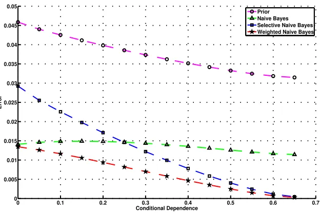
This example shows the relative performance of naive Bayes and weighted naive Bayes as we vary the conditional dependence between attributes. In particular it demonstrates how optimal assign-ment of weights will never result in higher error than attribute selection or standard naive Bayes, and that for certain violations of the attribute independence assumption it can result in lower error than either.
We will constrain ourselves to a binary class problem with two binary attributes. We quantify the conditional dependence between the attributes using the Conditional Mutual Information (CMI):
I(X1,X2|Y) =
∑
y
∑
x2∑
x1
P(x1,x2,y)log
P(x1,x2|y) P(x1|y)P(x2|y)
.
The results of varying the conditional dependence between the attributes on the performance of the different classifiers in terms of their Root Mean Squared Error (RMSE) is shown in Figure 1.
To generate these curves, we varied the probabilities P(y|x1,x2)and P(x1,x2)and plotted average results across distinct values of the Conditional Mutual Information. For each of the 4 possible attribute value combinations(x1,x2)∈ {(0,0),(0,1),(1,0),(1,1)}, we selected values for the class probability given the attribute value combination from the set: P(y|x1,x2)∈ {0.25,0.75}. Note that P(¬y|x1,x2) =1−P(y|x1,x2), so this process resulted in 24 possible assignments to the vector P(y|•,•).
0 0.1 0.2 0.3 0.4 0.5 0.6 0.7 0
0.005 0.01 0.015 0.02 0.025 0.03 0.035 0.04 0.045 0.05
Error
Conditional Dependence
Prior Naive Bayes Selective Naive Bayes Weighted Naive Bayes
Figure 1: Variation of Error of naive Bayes, selective naive Bayes, weighted naive Bayes and classi-fier based only on prior probabilities of the class as a function of conditional dependence (conditional mutual information) between the two attributes.
Pearson’s correlation coefficient, denotedρ, as follows:1
P(X1=0,X2=0) = P(X1=1,X2=1) =
(1+ρ) 4 , P(X1=0,X2=1) = P(X1=1,X2=0) =
(1−ρ) 4 , where −1≤ρ≤1.
Note that whenρ=−1 the attributes are perfectly anti-correlated (x1=¬x2), whenρ=0 the attributes are independent (since the joint distribution P(x1,x2)is uniform) and whenρ=1 the attributes are perfectly correlated.
For the graph, we increased values ofρin increments of 0.00004, resulting in 50000 distribu-tions (vectors) for P(•,•)for each vector P(y|•,•). Near optimal weights(w1,w2)for the weighted naive Bayes classifier were found using grid search over the range {{0.0,0.1,0.2, . . . ,0.9,1.0} ×
{0.0,0.1,0.2, . . . ,0.9,1.0}}. Results in Figure 1 are plotted by taking average across conditional mutual information values, with a window size of 0.1.
1. Note that from the definition of Pearson’s correlation coefficient we have:
ρ=p E[(X1−E[X1])(X2−E[X2])] E[(X1−E[X1])2]E[(X2−E[X2])2]
=4P(X1=1,X2=1)−1,
We compare the expected RMSE of naive Bayes (w1=1,w2=1), weighted naive Bayes, naive Bayes based on feature 1 only (selective Bayes withw1=1,w2=0), naive Bayes based on feature 2 only (selective Bayes withw1=0,w2=1), and naive Bayes using only the prior (equivalent to weighted naive Bayes with both weights set to 0.0). It can be seen that when conditional mutual information (CMI) is small, naive Bayes performs better than selective naive Bayes and the prior classifier. Indeed, when CMI is 0.0, naive Bayes is optimal. As CMI is increased, naive Bayes performance deteriorates compared to selective naive Bayes. Weighted naive Bayes, on the other hand, has the best performance in all circumstances. Due to the symmetry of the problem, the two selective Bayes classifiers give exactly the same results.
Note that in this experiment we have used the optimal weights to calculate the results. We have shown that weighted naive Bayes is capable ofexpressingmore accurate classifiers than selective naive Bayes. In the remaining sections we will examine and evaluate techniques for learning from data the weights those models require.
3. Survey of Attribute Weighting and Selecting Methods for Naive Bayes
Attribute weightingis well-understood in the context of nearest-neighbor learning methods and is used for reducing bias in high-dimensional problems due to the presence of redundant or irrelevant features (Friedman, 1994; Guyon et al., 2004). It is also used for mitigating the effects of the curse-of-dimensionality which results in exponential increase in the required training data as the number of features are increased (Bellman, 1957). Attribute weighting for naive Bayes is comparatively less explored.
Before discussing these techniques, however, it is useful to briefly examine the closely related area of feature selection for naive Bayes. As already pointed out, weighting can achieve feature selection by settings weights to either 0.0 or 1.0, and so can be viewed as a generalization of feature selection.
Langley and Sage (1994) proposed the Selective Bayes (SB) classifier, using feature selection to accommodate redundant attributes in the prediction process and to augment naive Bayes with the ability to exclude attributes that introduce dependencies. The technique is based on searching through the entire space of all attribute subsets. For that, they use a forward sequential search with a greedy approach to traverse the search space. That is, the algorithm initializes the subset of attributes to an empty set, and the accuracy of the resulting classifier, which simply predicts the most frequent class, is saved for subsequent comparison. On each iteration, the method considers adding each unused attribute to the subset on a trial basis and measures the performance of the resulting classifier on the training data. The attribute that most improves the accuracy is permanently added to the subset. The algorithm terminates when addition of any attribute results in reduced accuracy, at which point it returns the list of current attributes along with their ranks. The rank of the attribute is based on the order in which they are added to the subset.
The best subset found is returned when the search terminates. CFS uses a stopping criterion of five consecutive fully expanded non-improving subsets.
There has been a growing trend in the use of decision trees to improve the performance of other learning algorithms and naive Bayes classifiers are no exception. For example, one can build a naive Bayes classifier by using only those attributes appearing in a C4.5 decision tree. This is equivalent to giving zero weights to attributes not appearing in the decision tree. The Selective Bayesian Classifier (SBC) of Ratanamahatana and Gunopulos (2003) also employs decision trees for attribute selection for naive Bayes. Only those attributes appearing in the top three levels of a decision tree are selected for inclusion in naive Bayes. Since decision trees are inherently unstable, five decision trees (C4.5) are generated on samples generated by bootstrapping 10% from the training data. Naive Bayes is trained on an attribute set which comprises the union of attributes appearing in all five decision trees.
One of the earliest works on weighted naive Bayes is by Hilden and Bjerregaard (1976), who used weighting of the form of Equation 6. This strategy uses a single weight and therefore is not strictly performing attribute weighting. Their approach is motivated as a means of alleviating the effects of violations of the attribute independence assumption. Settingwto unity is appropriate when the conditional independence assumption is satisfied. However, on their data set (acute abdominal pain study in Copenhagen by Bjerregaard et al. 1976), improved classification was obtained whenw
was small, with an optimum value as low as 0.3. The authors point out that if symptom variables of a clinical field trial are not independent, but pair-wise correlated with independence between pairs, thenw=0.5 will be the correct choice since usingw=1 would make all probabilities the square of what they ought be. Looking at the optimal value ofw=0.3 for their data set, they suggested that out of ten symptoms, only three are providing independent information. The value of wwas obtained by maximizing the log-likelihood over the entire testing sample.
Zhang and Sheng (2004) used the gain ratio of an attribute with the class labels as its weight. Their formula is shown in Equation 7. The gain ratio is a well-studied attribute weighting tech-nique and is generally used for splitting nodes in decision trees (Duda et al., 2006). The weight of each attribute is set to the gain ratio of the attribute relative to the average gain ratio across all attributes. Note that, as a result of the definition at least one (possibly many) of the attributes have weights greater than 1, which means that they are not only attempting to lessen the effects of the independence assumption—otherwise they would restrict the weights to be no more than one.
wi=
GR(i) 1
a∑ a
i=1GR(i)
. (7)
The gain ratio of an attribute is then simply the Mutual Information between that attribute and the class label divided by the entropy of that attribute:
GR(i) = I(Xi,Y)
H(Xi)
=∑y∑x1P(x1,y)log P(x1,y)
P(x1)P(y) ∑x1P(x1)log
1 P(x1)
.
Several other wrapper-based methods are also proposed in Zhang and Sheng (2004). For example, they use a simple hill climbing search to optimize weightwusing Area Under Curve (AUC) as an evaluation metric. Another Markov-Chain-Monte-Carlo (MCMC) method is also proposed.
is randomly generated, weights in the population are constrained to be between 0 and 1. Second, typical genetic algorithmic steps of mutation and cross-over are performed over the the population. They defined a fitness function which is used to determine if mutation can replace the current in-dividual (weight vector) with a new one. Their algorithm employs a greedy search strategy, where mutated individuals are selected as offspring only if the fitness is better than that of target individual. Otherwise, the target is maintained in the next iteration.
A scheme used in Hall (2007) is similar in spirit to SBC where the weight assigned to each at-tribute is inversely proportional to the minimum depth at which they were first tested in an unpruned decision tree. Weights are stabilized by averaging across 10 decision trees learned on data samples generated by bootstrapping 50% from the training data. Attributes not appearing in the decision trees are assigned a weight of zero. For example, one can assign weight to an attributeias:
wi= 1
T T
∑
t
1
√
dti. (8)
where dti is the minimum depth at which the attribute iappears in decision treet, and T is the total number of decision trees generated. To understand whether the improvement in naive Bayes accuracy was due to attribute weighting or selection, a variant of the above approach was also proposed where all non-zero weights are set to one. This is equivalent to SBC except using a bootstrap size of 50% with 10 iterations.
Both SB and CFS are feature selection methods. Since selecting an optimal number of features is not trivial, Hall (2007) proposed to use SB and CFS for feature weighting in naive Bayes. For example, the weight of an attributeican be defined as:
wi=
1
√r
i
. (9)
whereri is the rank of the feature based on SB and CFS feature selection.
The feature weighting method proposed in Ferreira et al. (2001) is the only one to use Equa-tion 4, weighting each attribute value rather than each attribute. They used entropy-based dis-cretization for numeric attributes and assigned a weight to each partition (value) of the attribute that is proportional to its predictive capability of the class. Different weight functions are proposed to assign weights to the values. These functions measure the difference between the distribution over classes for the particular attribute-value pair and a “baseline class distribution”. The choice of weight function reduces to a choice of baseline distribution and the choice of measure quantifying the difference between the distributions. They used two simple baseline distribution schemes. The first assumes equiprobable classes, that is, uniform class priors. In that case the weight of for value
jof the attributeican be written as:
wi j ∝
∑
y
|P(y|Xi=j)− 1
|
Y
||α
!1/α
.
where P(y|Xi=j) denotes the probability that the class isy given that the i-th attribute of a data
point has value j. Alternatively, the baseline class distribution can be set to the class probabilities across all values of the attribute (i.e., the class priors). The weighing function will take the form:
wi j ∝
∑
y
|P(y|Xi=j)−P(y|Xi6=miss)|α
!1/α
where P(y|Xi6=miss) is the class prior probability across all data points for which the attributei
is not missing. Equation 10 and 10 assume anLαdistance metric whereα=2 corresponds to the
L2norm. Similarly, they have also proposed to use distance based on Kullback-Leibler divergence between the two distributions to set weights.
Many researchers have investigated techniques for extending the basic naive Bayes indepen-dence model with a small number of additional dependencies between attributes in order to im-prove classification performance (Zheng and Webb, 2000). Popular examples of suchsemi-naive Bayes methodsinclude Tree-Augmented Naive Bayes (TAN) (Friedman et al., 1997) and ensemble methods such as Averaged n-Dependence Estimators (AnDE) (Webb et al., 2011). While detailed discussion of these methods is beyond the scope of this work, we will describe both TAN and AnDE in Section 5.10 for the purposes of empirical comparison.
Semi-naive Bayes methods usually limit the structure of the dependency network to simple structures such as trees, but more general graph structures can also be learnt. Considerable research has been done in the area of learning general Bayesian Networks (Greiner et al., 2004; Grossman and Domingos, 2004; Roos et al., 2005), with techniques differing on whether the network structure is chosen to optimize a generative or discriminative objective function, and whether the same objective is also used for optimizing the parameters of the model. Indeed optimizing network structure using a discriminative objective function can quickly become computationally challenging and thus recent work in this area has looked at efficient heuristics for discriminative structure learning (Pernkopf and Bilmes, 2010) and at developing decomposable discriminative objective functions (Carvalho et al., 2011).
In this paper we are interested in improving performance of the NB classifier by reducing the effect of attribute independence violations through attribute weighting. We do not attempt to identify the particular dependencies between attributes that cause the violations and thus are not attempting to address the much harder problem of inducing the dependency network structure. While it is conceivable that semi-naive Bayes methods and more general Bayesian Network classifier learning could also benefit from attribute weighting, we leave its investigation to future work.
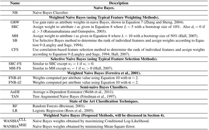
A summary of different methods compared in this research is given in Table 2.
4. Weighting to Alleviate the Naive Bayes Independence Assumption
In this section, we will discuss our proposed methods to incorporate weights in naive Bayes.
4.1 WANBIA
Name Description Naive Bayes.
NB Naive Bayes Classifier.
Weighted Naive Bayes (using Typical Feature Weighting Methods).
GRW Use gain ratio as attribute weights in naive Bayes, shown in Equation 7 (Zhang and Sheng, 2004).
SBC Assign weight to attributeias given in Equation 8 whereL=5 with a bootstrap size of 10%. Alsodi=0 if
di>3 (Ratanamahatana and Gunopulos, 2003).
MH Assign weight to attributeias given in Equation 8 whereL=10 with a bootstrap size of 50% (Hall, 2007). SB Use Selective Bayes method to determine the rank of individual features and assign weights according to
Equa-tion 9 (Langley and Sage, 1994).
CFS Use correlation-based feature selection method to determine the rank of individual features and assign weights according to Equation 9 (Langley and Sage, 1994; Hall, 2007).
Selective Naive Bayes (using Typical Feature Selection Methods).
SBC-FS Similar to SBC exceptwi=1 ifwi>0.
MH-FS Similar to MH exceptwi=1 ifwi>0 (Hall, 2007).
Weighted Naive Bayes (Ferreira et al., 2001).
FNB-d1 Weights computed per attribute value using Equation 10 withα=2. FNB-d2 Weights computed per attribute value using Equation 10 withα=2.
Semi-naive Bayes Classifiers.
AnDE Averagen-Dependent Estimator (Webb et al., 2011). TAN Tree Augmented Naive Bayes (Friedman et al., 1997).
State of the Art Classification Techniques.
RF Random Forests (Breiman, 2001). LR Logistic Regression (Roos et al., 2005).
Weighted Naive Bayes (Proposed Methods, will be discussed in Section 4).
WANBIACLL Naive Bayes weights obtained by maximizing Conditional Log-Likelihood. WANBIAMSE Naive Bayes weights obtained by minimizing Mean-Square-Error.
Table 2: Summary of techniques compared in this research.
reduce the accuracy of the classifier relative to using uniform weights in any situation wherex1and
x3receive higher weights thanx2.
Rather than selecting weights based on measures of predictiveness, we suggest it is more prof-itable to pursue approaches such as those of Zhang and Sheng (2004) and Wu and Cai (2011) that optimize the weights to improve the prediction performance of the weighted classifier as a whole.
Following from Equations 1, 2 and 5, let us re-define the weighted naive Bayes model as:
ˆP(y|x;π,Θ,w) = πy∏iθ
wi
Xi=xi|y
∑y′πy′∏iθwXi
i=xi|y′
, (10)
with constraints:
∑yπy=1 and ∀y,i∑jθXi=xi|y=1, where
• {πy,θXi=xi|y}are naive Bayes parameters.
• π∈[0,1]|Y| is a class probability vector.
• The matrixΘconsist of class and attribute-dependent probability vectorsθi,y∈[0,1]|Xi|.
Our proposed method WANBIA is inspired by Cerquides and De M´antaras (2005b) where weights of different classifiers in an ensemble are calculated by maximizing the conditional log-likelihood (CLL) of the data. We will follow their approach of maximizing the CLL of the data to determine weightswin the model. In doing so, we will make the following assumptions:
• Naive Bayes parameters (πy,θXi=xi|y) are fixed. Hence we can write ˆP(y|x;π,Θ,w)in Equa-tion 10 as ˆP(y|x;w).
• Weights lie in the interval between zero and one and hencew∈[0,1]a.
For notational simplicity, we will write conditional probabilities asθxi|y instead ofθXi=xi|y. Since our prior is constant, let us define our supervised posterior as follows:
ˆP(
L
|D,
w) =|D|
∏
j=1
ˆP(y(j)|x(j);w). (11)
Taking the log of Equation 11, we get the Conditional Log-Likelihood (CLL) function, so our objective function can be defined as:
CLL(w) = log ˆP(
L
|D,
w) (12)=
|D|
∑
j=1
log ˆP(y(j)|x(j);w)
=
|D|
∑
j=1
log γyx(w)
∑y′γy′x(w),
where
γyx(w) =πy
∏
iθwi
xi|y.
The proposed method WANBIACLL is aimed at solving the following optimization problem: find the weightswthat maximizes the objective function CLL(w) in Equation 12 subject to 0≤wi≤
1 ∀i. We can solve the problem by using the L-BFGS-M optimization procedure (Zhu et al., 1997). In order to do that, we need to be able to assess CLL(w)in Equation 12 and its gradient.
Before calculating the gradient of CLL(w) with respect to w, let us find out the gradient of
γyx(w)with respect towi, we can write:
∂ ∂wi
γyx(w) = (πy
∏
i′6=iθwi′
xi′|y)
∂ ∂wi
θwi
xi|y
= (πy
∏
i′6=i θwi′
xi′|y)θ
wi
xi|ylog(θxi|y)
= γyx(w)log(θxi|y). (13)
Now, we can write the gradient of CLL(w)as:
∂ ∂wi
CLL(w) = ∂
∂wix
∑
∈Dlog(γyx(w))−log(
∑
y′
γy′x(w))
=
∑
x∈D
γ
yx(w)log(θxi|y)
γyx(w) −
∑y′γy′x(w)log(θxi|y′) ∑y′γy′x(w)
=
∑
x∈D
log(θxi|y)−
∑
y′
ˆP(y′|x;w)log(θxi|y′)
!
. (14)
WANBIACLL evaluates the function in Equation 12 and its gradient in Equation 14 to determine optimal values of weight vectorw.
Instead of maximizing the supervised posterior, one can also minimize Mean Square Error (MSE). Our second proposed weighting scheme WANBIAMSE is based on minimizing the MSE function. Based on MSE, we can define our objective function as follows:
MSE(w) =1
2
∑
x(j)∈D
∑
y(P(y|x(j))−ˆP(y|x(j)))2, (15)
where we define
P(y|x(j)) =
1 ify=y(j)
0 otherwise .
The gradient of MSE(w)in Equation 15 with respect towcan be derived as:
∂MSE(w)
∂wi
=−
∑
x∈D
∑
yP(y|x)−ˆP(y|x)∂ˆP(y|x)
∂wi
, (16)
where
∂ˆP(y|x)
∂wi =
∂ ∂wiγyx(w)
∑y′γy′x(w)−
γyx(w)∂∂wi∑y′γy′x(w)
(∑y′γy′x(w))2
= 1
∑y′γy′x(w)
∂γyx(w)
∂wi −ˆP(y|x)
∑
y′∂γy′x(w) ∂wi
!
.
Following from Equation 13, we can write:
∂ˆP(y|x)
∂wi
= 1
∑y′γy′x(w) γyx(w)log(θxi|y)−
ˆP(y|x)
∑
y′
γy′x(w)log(θxi|y′)
!
= ˆP(y|x)log(θxi|y)−ˆP(y|x)
∑
y′
ˆP(y′|x)log(θxi|y′)
= ˆP(y|x) log(θxi|y)−
∑
y′
ˆP(y′|x)log(θxi|y′)
!
. (17)
Plugging the value of ∂ˆP∂(wy|x)
i from Equation 17 in Equation 16, we can write the gradient as:
∂MSE(w)
∂wi = −x
∑
∈D∑
y P(y|x)−ˆP(y|x)ˆP(y|x)
log(θxi|y)−
∑
y′
ˆP(y′|x)log(θxi|y′)
!
WANBIAMSE evaluates the function in Equation 15 and its gradient in Equation 18 to determine the optimal value of weight vectorw.
4.2 Connections with Logistic Regression
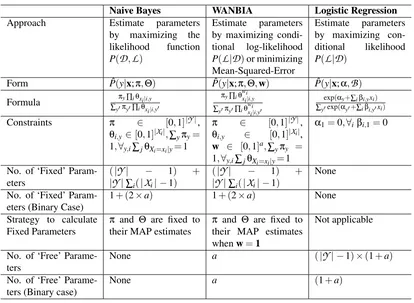
In this section, we will re-visit naive Bayes to illustrate WANBIA’s connection with the logistic regression.
4.2.1 BACKGROUND: NAIVEBAYES ANDLOGISTICREGRESSION
As discussed in Section 2 and 4.1, the naive Bayes (NB) model for estimating P(y|x) is parame-terized by a class probability vectorπ∈[0,1]|Y| and a matrixΘ, consisting of class and attribute
dependent probability vectorsθi,y∈[0,1]|Xi|. The NB model thus contains
(|
Y
| −1) +|Y
|∑
i
(|
X
i| −1)free parameters, which are estimated by maximizing the likelihood function: P(
D,
L
;π,Θ) =∏
j
P(y(j),x(j)),
or the posterior over model parameters (in which case they are referred to as maximum a posteriori or MAP estimates). Importantly, these estimates can be calculated analytically from attribute-value count vectors.
Meanwhile a multi-class logistic regression model is parameterized by a vectorα∈
R
|Y| andmatrix
B
∈R
|Y|×aeach consisting of real values, and can be written as:PLR(y|x;α,B) = exp(αy+∑iβi,yxi)
∑y′exp(αy′+∑iβi,y′xi),
where
α1=0 & ∀iβi,1=0.
The constraints arbitrarily setting all parameters fory=1 to the value zero are necessary only to prevent over-parameterization. The LR model, therefore, has:
(|
Y
| −1)×(1+a)free parameters. Rather than maximizing the likelihood, LR parameters are estimated by maximiz-ing the conditional likelihood of the class labels given the data:
P(
L
|D
;α,B) =∏
j
P(y(j)|x(j)),
or the corresponding posterior distribution. Estimating the parameters in this fashion requires search using gradient-based methods.
by simply looking up the corresponding parameter θXi=xi|y in Θ, while for LR it is calculated as exp(βi,yxi), that is, by taking the exponent of the product of the value with an attribute (but not
value) dependent parameterβi,y from
B
.24.2.2 PARAMETERS OFWEIGHTEDATTRIBUTENAIVEBAYES
The WANBIA model is an extension of the NB model where we introduce a weight vectorw∈[0,1]a
containing a class-independent weightwifor each attributei. The model as written in Equation 10
includes the NB model as a special case (where w=1). We do not treat the NB parameters of the model as free however, but instead fix them to their MAP estimates (assuming the weights were all one), which can be computed analytically and therefore does not require any search. We then estimate the parameter vectorwby maximizing the Conditional Log Likelihood (CLL) or by minimizing the Mean Squared Error (MSE).3
Thus in terms of the number of parameters that needs to be estimated using gradient-based search, a WANBIA model can be considered to haveafree parameters, which is always less than the corresponding LR model with(|
Y
| −1)(1+a)free parameters to be estimated. Thus for a binary class problems containing only binary attributes, WANBIA has 1 less free parameter than LR, but for multi-class problems with binary attributes it results in amultiplicative factorof |Y
| −1 fewer parameters. Since parameter estimation using CLL or MSE (or even Hinge Loss) requires search, fewer free parameters to estimate means faster learning and therefore scaling to larger problems.For problems containing non-binary attributes, WANBIA allows us to build (more expressive)
non-linear classifiers, which are not possible for Logistic Regression unless one “binarizes” all attributes, with the resulting blow-out in the number of free parameters as mentioned above. One should note that LR can only operate on nominal data by binarizing it. Therefore, on discrete problems with nominal data, WANBIA offers significant advantage in terms of the number of free parameters.
Lest the reader assume that the only goal of this work is to find a more computationally effi-cient version of LR, we note that the real advantage of the WANBIA model is to make use of the information present in the easy to compute naive Bayes MAP estimates to guide the search toward reasonable settings for parameters of a model that isnot hampered by the assumption of attribute independence.
A summary of the comparison of naive Bayes, WANBIA and Logistic Regression is given in Table 3.
5. Experiments
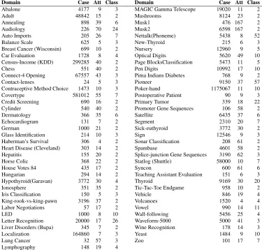
In this section, we compare the performance of our proposed methods WANBIACLL and WANBIAMSE with state of the art classifiers, existing semi-naive Bayes methods and weighted naive Bayes methods based on both attribute selection and attribute weighting. The performance is analyzed in terms of 0-1 loss, root mean square error (RMSE), bias and variance on 73 natural do-mains from the UCI repository of machine learning (Frank and Asuncion, 2010). Table 4 describes the details of each data set used, including the number of instances, attributes and classes.
2. Note that unlike the NB model, the LR model does not require that the domain of attribute values be discrete. Non-discrete data can also be handled by Naive Bayes models, but a different parameterization for the distribution over attribute values must be used.
Naive Bayes WANBIA Logistic Regression Approach Estimate parameters
by maximizing the likelihood function P(D,L)
Estimate parameters by maximizing condi-tional log-likelihood P(L|D)or minimizing Mean-Squared-Error
Estimate parameters by maximizing con-ditional likelihood P(L|D)
Form Pˆ(y|x;π,Θ) Pˆ(y|x;π,Θ,w) Pˆ(y|x;α,B)
Formula ∑πy∏iθxi|i,y y′πy′∏iθxi|i,y′
πy∏iθwixi|i,y
∑y′πy′∏iθwixi|i,y′
exp(αy+∑iβi,yxi)
∑y′exp(αy′+∑iβi,y′xi) Constraints π ∈ [0,1]|Y|,
θi,y∈[0,1]|Xi|,∑yπy=
1,∀y,i∑jθXi=xi|y=1
π ∈ [0,1]|Y|,
θi,y ∈ [0,1]|Xi|,
w ∈ [0,1]a,∑yπy =
1,∀y,i∑jθXi=xi|y=1
α1=0,∀iβi,1=0
No. of ‘Fixed’ Param-eters
(|Y| − 1) +
|Y|∑i(|Xi| −1)
(|Y| − 1) +
|Y|∑i(|Xi| −1)
None
No. of ‘Fixed’ Param-eters (Binary Case)
1+ (2×a) 1+ (2×a) None Strategy to calculate
Fixed Parameters
π and Θ are fixed to their MAP estimates
π and Θ are fixed to their MAP estimates whenw=1
Not applicable
No. of ‘Free’ Parame-ters
None a (|Y| −1)×(1+a)
No. of ‘Free’ Parame-ters (Binary case)
None a (1+a)
Table 3: Comparison of naive Bayes, weighted naive Bayes and Logistic Regression
This section is organized as follows: we will discuss our experimental methodology with details on statistics employed and miscellaneous issues in Section 5.1. Section 5.2 illustrates the impact of a single weight on bias, variance, 0-1 loss and RMSE of naive Bayes as shown in Equation 6. The performance of our two proposed weighting methods WANBIACLL and WANBIAMSE is compared in Section 5.3. We will discuss the calibration performance of WANBIA in Section 5.4. In Section 5.5, we will discuss results when the proposed methods are constrained to learn only a single weight. In Section 5.6 and 5.7, WANBIACLL and WANBIAMSE are compared with naive Bayes where weights are induced through various feature weighting and feature selection schemes respectively. We compare the performance of our proposed methods with per-attribute value weight learning method of Ferreira et al. (2001) in Section 5.8. We will discuss the significance of these results in Section 5.9. The performance of our proposed methods is compared with state of the art classifiers like Average n-Dependent Estimators (AnDE), Tree Augmented Networks (TAN), Random Forests (RF) and Logistic Regression (LR) in Section 5.10, 5.11 and 5.12 respectively. Results are summarized in Section 5.13.
5.1 Experimental Methodology
Domain Case Att Class Domain Case Att Class
Abalone 4177 9 3 MAGIC Gamma Telescope 19020 11 2
Adult 48842 15 2 Mushrooms 8124 23 2
Annealing 898 39 6 Musk1 476 167 2
Audiology 226 70 24 Musk2 6598 167 2
Auto Imports 205 26 7 Nettalk(Phoneme) 5438 8 52
Balance Scale 625 5 3 New-Thyroid 215 6 3
Breast Cancer (Wisconsin) 699 10 2 Nursery 12960 9 5
Car Evaluation 1728 8 4 Optical Digits 5620 49 10
Census-Income (KDD) 299285 40 2 Page BlocksClassification 5473 11 5
Chess 551 40 2 Pen Digits 10992 17 10
Connect-4 Opening 67557 43 3 Pima Indians Diabetes 768 9 2
Contact-lenses 24 5 3 Pioneer 9150 37 57
Contraceptive Method Choice 1473 10 3 Poker-hand 1175067 11 10
Covertype 581012 55 7 Postoperative Patient 90 9 3
Credit Screening 690 16 2 Primary Tumor 339 18 22
Cylinder 540 40 2 Promoter Gene Sequences 106 58 2
Dermatology 366 35 6 Satellite 6435 37 6
Echocardiogram 131 7 2 Segment 2310 20 7
German 1000 21 2 Sick-euthyroid 3772 30 2
Glass Identification 214 10 3 Sign 12546 9 3
Haberman’s Survival 306 4 2 Sonar Classification 208 61 2
Heart Disease (Cleveland) 303 14 2 Spambase 4601 58 2
Hepatitis 155 20 2 Splice-junction Gene Sequences 3190 62 3
Horse Colic 368 22 2 Statlog (Shuttle) 58000 10 7
House Votes 84 435 17 2 Syncon 600 61 6
Hungarian 294 14 2 Teaching Assistant Evaluation 151 6 3
Hypothyroid(Garavan) 3772 30 4 Thyroid 9169 30 20
Ionosphere 351 35 2 Tic-Tac-Toe Endgame 958 10 2
Iris Classification 150 5 3 Vehicle 846 19 4
King-rook-vs-king-pawn 3196 37 2 Volcanoes 1520 4 4
Labor Negotiations 57 17 2 Vowel 990 14 11
LED 1000 8 10 Wall-following 5456 25 4
Letter Recognition 20000 17 26 Waveform-5000 5000 41 3 Liver Disorders (Bupa) 345 7 2 Wine Recognition 178 14 3
Localization 164860 7 3 Yeast 1484 9 10
Lung Cancer 32 57 3 Zoo 101 17 7
Lymphography 148 19 4
Table 4: Data sets
of each algorithm. The experiments were conducted on a Linux machine with 2.8 GHz processor and 16 GB of RAM.
5.1.1 TWO-FOLDCROSS-VALIDATION BIAS-VARIANCEESTIMATION
The Bias-variance decomposition provides valuable insights into the components of the error of learned classifiers. Biasdenotes the systematic component of error, which describes how closely the learner is able to describe the decision surfaces for a domain.Variancedescribes the component of error that stems from sampling, which reflects the sensitivity of the learner to variations in the training sample (Kohavi and Wolpert, 1996; Webb, 2000). There are a number of different bias-variance decomposition definitions. In this research, we use the bias and bias-variance definitions of Kohavi and Wolpert (1996) together with the repeated cross-validation bias-variance estimation method proposed by Webb (2000). Kohavi and Wolpert define bias and variance as follows:
bias2= 1
2y
∑
∈Y P(y|x)−ˆP(y|x) 2and
variance=1
2 1−y
∑
∈Y
ˆP(y|x)2 !
.
In the method of Kohavi and Wolpert (1996), which is the default bias-variance estimation method in Weka, the randomized training data are randomly divided into a training pool and a test pool. Each pool contains 50% of the data. 50 (the default number in Weka) local training sets, each containing half of the training pool, are sampled from the training pool. Hence, each local training set is only 25% of the full data set. Classifiers are generated from local training sets and bias, variance and error are estimated from the performance of the classifiers on the test pool. However, in this work, the repeated cross-validation bias-variance estimation method is used as it results in the use of substantially larger training sets. Only two folds are used because, if more than two are used, the multiple classifiers are trained from training sets with large overlap, and hence the estimation of variance is compromised. A further benefit of this approach relative to the Kohavi Wolpert method is that every case in the training data is used the same number of times for both training and testing. A reason for performing bias/variance estimation is that it provides insights into how the learn-ing algorithm will perform with varylearn-ing amount of data. We expect low variance algorithms to have relatively low error for small data and low bias algorithms to have relatively low error for large data (Damien and Webb, 2002).
5.1.2 STATISTICSEMPLOYED
We employ the following statistics to interpret results:
• Win/Draw/Loss (WDL) Record -When two algorithms are compared, we count the number of data sets for which one algorithm performs better, equally well or worse than the other on a given measure. A standard binomial sign test, assuming that wins and losses are equiprobable, is applied to these records. We assess a difference as significant if the outcome of a one-tailed binomial sign test is less than 0.05.
• Average -The average (arithmetic mean) across all data sets provides a gross indication of relative performance in addition to other statistics. In some cases, we normalize the results with respect to one of our proposed method’s results and plot the geometric mean of the ratios.
• Significance (Friedman and Nemenyi) Test -We employ the Friedman and the Nemenyi tests for comparison of multiple algorithms over multiple data sets (Demˇsar, 2006; Friedman, 1937, 1940). The Friedman test is a non-parametric equivalent of the repeated measures ANOVA (analysis of variance). We follow the steps below to compute results:
– Calculate the rank of each algorithm for each data set separately (assign average ranks in case of a tie). Calculate the average rank of each algorithm.
– Compute the Friedman statistics as derived in Kononenko (1990) for the set of average ranks:
FF =
(D−1)χ2
F D(g−1)−χ2
F
where
χ2F= 12D
g(g+1)
∑
i R 2i −
g(g+1)2 4
!
,
gis the number of algorithms being compared,Dis the number of data sets andRiis the average rank of thei-th algorithm.
– Specify the null hypothesis. In our case the null hypothesis is that there is no difference in the average ranks.
– Check if we can reject the null hypothesis. One can reject the null hypothesis if the Friedman statistic (Equation 19) is larger than the critical value of the F distribution withg−1 and(g−1)(D−1)degrees of freedom forα=0.05.
– If null hypothesis is rejected, perform Nemenyi tests which is used to further analyze which pairs of algorithms are significantly different. Letdi j be the difference between the average ranks of theith algorithm and jth algorithm. We assess the difference be-tween the algorithms to be significant ifdi j>critical difference(CD)=q0.05
q
g(g+1)
6D ,
whereq0.05 are the critical values that are calculated by dividing the values in the row for the infinite degree of freedom of the table of Studentized range statistics (α=0.05) by√2.
5.1.3 MISCELLANEOUSISSUES
This section explains other issues related to the experiments.
• Probability Estimates - The base probabilities of each algorithm are estimated using m -estimation, since in our initial experiments it leads to more accurate probabilities than Laplace estimation for naive Bayes and weighted naive Bayes. In the experiments, we usem=1.0, computing the conditional probability as:
ˆP(xi|y) =
Nxi,y+
m
|Xi| (Ny−N?) +m
, (20)
whereNxi,y is the count of data points with attribute valuexi and class labely,Nyis the count of data points with class labely,N?is the number of missing values of attributei.
• Numeric Values -To handle numeric attributes we tested the following techniques in our initial experiments:
– Quantitative attributes are discretized using three bin discretization.
– Quantitative attributes are discretized using Minimum Description Length (MDL) dis-cretization (Fayyad and Keki, 1992).
– Kernel Density Estimation (KDE) computing the probability of numeric attributes as:
ˆP(xi|y) =1
n
∑
x(j)∈D
exp ||x
j i−xi||2
λ2 !
NB vs. NBw
W/D/L w=0.1 w=0.2 w=0.3 w=0.4 w=0.5 w=0.6 w=0.7 w=0.8 w=0.9 w=1.0
0/1 Loss 61/2/10 58/1/14 53/1/19 51/3/19 46/3/24 39/5/29 36/8/29 28/11/34 23/12/38 0/73/0
<0.001 <0.001 <0.001 <0.001 0.011 0.532 0.457 0.525 0.072 2
NB vs. NBw
W/D/L w=0.1 w=0.2 w=0.3 w=0.4 w=0.5 w=0.6 w=0.7 w=0.8 w=0.9 w=1.0
RMSE 53/1/19 44/1/28 37/1/35 26/1/46 21/1/51 18/1/54 17/1/55 13/1/59 12/2/59 0/73/0
<0.001 0.076 0.906 0.024 <0.001 <0.001 <0.001 <0.001 <0.001 2
NB vs. NBw
W/D/L w=0.1 w=0.2 w=0.3 w=0.4 w=0.5 w=0.6 w=0.7 w=0.8 w=0.9 w=1.0
Bias 59/2/12 54/1/18 51/3/19 49/3/21 48/5/20 44/4/25 43/6/24 35/9/29 29/14/30 0/73/0
<0.001 <0.001 <0.001 <0.001 <0.001 0.029 0.027 0.532 1 2
NB vs. NBw
W/D/L w=0.1 w=0.2 w=0.3 w=0.4 w=0.5 w=0.6 w=0.7 w=0.8 w=0.9 w=1.0
Variance 39/1/33 38/3/32 30/7/36 31/4/38 30/6/37 31/4/38 23/11/39 22/18/33 25/18/30 0/73/0
0.556 0.550 0.538 0.470 0.463 0.470 0.055 0.177 0.590 2 Table 5: Win/Draw/Loss comparison of NB with weighted NB of form Equation 6
– k-Nearest neighbor (k-NN) estimation to compute the probability of numeric attributes. The probabilities are computed using Equation 20, where Nxi,y and Ny are calculated over a neighborhood spanningkneighbors ofxi. We usek=10,k=20 andk=30.
While a detailed analysis of the results of this comparison is beyond the scope of this work, we summarize our findings as follows: the k-NN approach with k=50 achieved the best 0-1 loss results in terms of Win/Draw/Loss. The k-NN withk=20 resulted in the best bias performance, KDE in the best variance and MDL discretization in best RMSE performance. However, we found KDE and k-NN schemes to be extremely slow at classification time. We found that MDL discretization provides the best trade-off between the accuracy and compu-tational efficiency. Therefore, we chose to discretize numeric attributes with MDL scheme.
• Missing Values - For the results reported in from Section 5.2 to Section 5.9, the missing val-ues of any attributes are incorporated in probability computation as depicted in Equation 20. Starting from Section 5.10, missing values are treated as a distinct value. The motivation be-hind this is to have a fair comparison between WANBIA and other state of the art classifiers, for instance, Logistic Regression and Random Forest.
• Notation -We will categorize data sets in terms of their size. For example, data sets with in-stances≤1000,>1000 and≤10000,>10000 are denoted as bottom size, medium size and top size respectively. We will report results on these sets to discuss suitability of a classifier for data sets of different sizes.
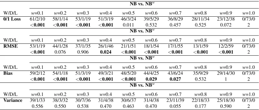
5.2 Effects of a Single Weight on Naive Bayes
terms of 0-1 loss and RMSE and non-significantly better performance in terms of bias and variance as compared to the lower values.
Averaged (arithmetic mean) 0-1 loss, RMSE, bias and variance results across 73 data sets as a function of weight are plotted in Figure 2 and 3. As can be seen from the figures that as w
0.1 0.2 0.3 0.4 0.5 0.6 0.7 0.8 0.9 1
0.2 0.21 0.22 0.23 0.24 0.25 0.26 0.27 0.28
0/1 Loss
(a)
0.1 0.2 0.3 0.4 0.5 0.6 0.7 0.8 0.9 1 0.27
0.28 0.29 0.3 0.31 0.32
RMSE
(b)
Figure 2: Averaged 0-1 Loss (2(a)), RMSE (2(b)) across 73 data sets, as function ofw.
0.1 0.2 0.3 0.4 0.5 0.6 0.7 0.8 0.9 1 0.16
0.17 0.18 0.19 0.2 0.21 0.22 0.23 0.24
Bias
(a)
0.1 0.2 0.3 0.4 0.5 0.6 0.7 0.8 0.9 1
0.04 0.042 0.044 0.046 0.048 0.05 0.052
Variance
(b)
Figure 3: Averaged Bias (3(a)) Variance (3(b)) across 73 data sets, as function ofw.
is increased from 0.1 to 1.0, bias decreases and variance increases. It is hard to characterize 0-1 loss and RMSE curves in Figure 2. 0-1 loss is decreased as we increase the value of w and is almost constant whenw>0.7. However, RMSE drops aswis increased to 0.5 and then increases forw>0.5. As the results are averaged across 73 data sets, it is hard to say anything conclusive, however, we conjecture that the optimal value of 0.5 forwin case of RMSE metric suggests that in most data sets, only half of the attributes are providing independent information.
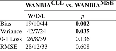
5.3 Mean-Square-Error versus Conditional-Log-Likelihood Objective Function
WANBIACLL vs. WANBIAMSE
W/D/L p
Bias 19/10/44 0.002
Variance 42/7/24 0.035
0-1 Loss 26/8/39 0.136
RMSE 28/12/33 0.608
Table 6: Win/Draw/Loss: WANBIACLL versus WANBIAMSE
WANBIACLL vs. NB WANBIAMSE vs. NB
W/D/L p W/D/L p
Bias 55/7/11 <0.001 57/7/9 <0.001
Variance 24/8/41 0.046 24/7/42 0.035
0-1 Loss 46/8/19 0.001 49/7/17 <0.001
RMSE 55/8/10 <0.001 54/6/13 <0.001
Table 7: Win/Draw/Loss: WANBIACLL versus NB, WANBIAMSE versus NB
Since the performance of WANBIAMSE and WANBIACLL is similar, from the following section onwards, for simplicity we will only consider WANBIAMSE when comparing with other weighted NB and state of the art classification methods and denote it by WANBIA.
5.4 Comparing the Calibration of WANBIA and NB Probability Estimates
One benefit of Bayesian classifiers (and indeed also Logistic Regression) over Support Vector Ma-chine and Decision-Tree based classifiers is that the former implicitly produce interpretable confi-dence values for each classification in the form of class membership probability estimates ˆP(y|x). Unfortunately, the probability estimates that naive Bayes produces can often be poorly calibrated as a result of the conditional independence assumption. Whenever the conditional independence as-sumption is violated, which is usually the case in practice, the probability estimates tend to be more extreme (closer to zero or one) than they should otherwise be. In other words, the NB classifier tends to be more confident in its class membership predictions than is warranted given the training data. Poor calibration and over-confidence do not always affect performance in terms of 0-1 Loss, but in many applications accurate estimates of the probability ofxbelonging to classyare needed (Zadrozny and Elkan, 2002).
Since, WANBIA is based on alleviating the attribute-independence assumption, it also corrects for naive Bayes’ poor calibration as can be seen in Figure 4.
Figure 4 shows reliability diagrams showing the relative calibration for naive Bayes and WANBIA (DeGroot and Fienbert, 1982). Reliability diagrams plot empirical class membership probability
˜P(y|ˆP(y|x))versus predicted class membership probability for ˆP(y|x)at various levels of the latter. If a classifier is well-calibrated, all points will lie on the diagonal indicating that estimates are equal to their empirical probability. In the diagrams, the empirical probability ˜P(y|ˆP(y|x) =p)is the ratio of the number of training points with predicted probabilitypbelonging to classyto the total number of training points with predicted probability p. Since, the number of different predicted values is large as compared to the number of data points, we can not calculate reliable empirical probabilities for each data point, but instead bin the predicted values along the x-axis. For plots in Figure 4, we have used a bin size of 0.05.
Reliability diagrams are shown for sample data sets Adult, Census-income, Connect-4, Local-ization, Magic, Page-blocks, Pendigits, Satellige and Sign. One can see that WANBIA often attains far better calibrated class membership probability estimates.
0 0.1 0.2 0.3 0.4 0.5 0.6 0.7 0.8 0.9 1 0 0.1 0.2 0.3 0.4 0.5 0.6 0.7 0.8 0.9 1 Predicted Probability
Empirical class membership probability
Adult
NB WANBIA
0 0.1 0.2 0.3 0.4 0.5 0.6 0.7 0.8 0.9 1 0 0.1 0.2 0.3 0.4 0.5 0.6 0.7 0.8 0.9 1 Predicted Probability
Empirical class membership probability
Census−income
NB WANBIA
0 0.1 0.2 0.3 0.4 0.5 0.6 0.7 0.8 0.9 1 0 0.1 0.2 0.3 0.4 0.5 0.6 0.7 0.8 0.9 1 Predicted Probability
Empirical class membership probability
Connect−4
NB WANBIA
0 0.1 0.2 0.3 0.4 0.5 0.6 0.7 0.8 0.9 1 0 0.1 0.2 0.3 0.4 0.5 0.6 0.7 0.8 0.9 1 Predicted Probability
Empirical class membership probability
Localization NB
WANBIA
0 0.1 0.2 0.3 0.4 0.5 0.6 0.7 0.8 0.9 1 0 0.1 0.2 0.3 0.4 0.5 0.6 0.7 0.8 0.9 1 Predicted Probability
Empirical class membership probability
Magic NB
WANBIA
0 0.1 0.2 0.3 0.4 0.5 0.6 0.7 0.8 0.9 1
0 0.1 0.2 0.3 0.4 0.5 0.6 0.7 0.8 0.9 1 Predicted Probability
Empirical class membership probability
Page−blocks
NB WANBIA
0 0.1 0.2 0.3 0.4 0.5 0.6 0.7 0.8 0.9 1
0 0.1 0.2 0.3 0.4 0.5 0.6 0.7 0.8 0.9 1 Predicted Probability
Empirical class membership probability
Pendigits
NB WANBIA
0 0.1 0.2 0.3 0.4 0.5 0.6 0.7 0.8 0.9 1
0 0.1 0.2 0.3 0.4 0.5 0.6 0.7 0.8 0.9 1 Predicted Probability
Empirical class membership probability
Satellite
NB WANBIA
0 0.1 0.2 0.3 0.4 0.5 0.6 0.7 0.8 0.9 1
0 0.1 0.2 0.3 0.4 0.5 0.6 0.7 0.8 0.9 1 Predicted Probability
Empirical class membership probability
Sign
NB WANBIA
Figure 4: Reliability diagrams of naive Bayes and WANBIA on nine data sets.
5.5 Single versus Multiple Naive Bayes Weights Learning
To study the effect of single versus multiple weight learning for naive Bayes (naive Bayes in Equa-tion 5 versus naive Bayes in EquaEqua-tion 6), we constrained WANBIA to learn only a single weight for all attributes. The method is denoted by WANBIA-S and compared with WANBIA and naive Bayes in Table 8.
vs. WANBIA vs. NB
W/D/L p W/D/L p
Bias 5/7/61 <0.001 27/18/28 1 Variance 46/7/20 0.001 29/21/23 0.488 0-1 Loss 17/7/49 <0.001 30-18/25 0.590 RMSE 19/7/47 <0.001 52/15/6 <0.001
Table 8: Win/Draw/Loss: WANBIA-S vs. WANBIA and NB
the effect of the bias-variance trade-off. Learning multiple weights result in lowering the bias but increases the variance of classification. As can be seen from the table, the performance of WANBIA-S compared to NB is fairly even in terms of 0-1 loss, bias and variance and WDL re-sults are non-significant. However, RMSE is significantly improved as WANBIA-S improves naive Bayes probability estimates on 52 of the 73 data sets.
5.6 WANBIA versus Weighted Naive Bayes Using Feature Weighting Methods
The Win/Draw/Loss results of WANBIA against GRW, SBC, MH and CFS weighting NB tech-niques are given in Table 9. It can be seen that WANBIA has significantly better 0-1 loss, bias and RMSE than all other methods. Variance is, however, worst comparing to GRW, CFS and SB.
vs. GRW vs. SBC vs. MH vs. CFS vs. SB
Bias 60/0/13 64/1/8 62/3/8 63/4/6 61/5/7
p <0.001 0.048 <0.001 0.048 <0.001
Variance 31/1/41 46/1/26 28/2/43 21/4/48 29/3/41
p 0.288 0.012 0.095 0.001 0.188 0-1 Loss 58/0/15 66/1/6 57/2/14 50/3/20 52/3/18
p <0.001 <0.001 <0.001 <0.001 <0.001
RMSE 65/1/7 62/2/9 54/2/17 50/4/19 52/3/18
p <0.001 <0.001 <0.001 <0.001 <0.001
Table 9: Win/Draw/Loss: WANBIA versus Feature Weighting Methods
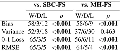
5.7 WANBIA versus Selective Naive Bayes
In this section, we will compare WANBIA performance with that of selective naive Bayes classifiers SBC-FS and MH-FS. The Win/Draw/Loss results are given in Table 10. It can be seen that WANBIA has significantly better 0-1 loss, bias and RMSE as compared to SBC-FS and MH-FS. It also has better variance as compared to the other methods.
5.8 WANBIA versus Ferreira et al. Approach
vs. SBC-FS vs. MH-FS
W/D/L p W/D/L p
Bias 58/3/12 <0.001 58/6/9 <0.001
Variance 52/3/18 <0.001 37/6/30 0.463 0-1 Loss 65/3/5 <0.001 56/6/11 <0.001
RMSE 65/3/5 <0.001 64/5/4 <0.001
Table 10: Win/Draw/Loss: WANBIACLL, WANBIAMSE vs. SBC-FS and MH-FS
vs. FNB-d1 vs. FNB-d2
W/D/L p W/D/L p
Bias 70/2/1 <0.001 64/1/8 <0.001
Variance 27/3/43 0.072 30/1/42 0.194 0-1 Loss 58/2/13 <0.001 59/1/13 <0.001
RMSE 56/1/16 <0.001 59/1/13 <0.001
Table 11: Win/Draw/Loss: WANBIA vs. FNB-d1 and FNB-d2
5.9 Discussion
In this section, we discuss the significance of the results presented in the Sections 5.6, 5.7 and 5.8 using Friedman and Nemenyi tests. Following the graphical representation of Demˇsar (2006), we show the comparison of techniques WANBIA, GRW, SBC, MH, CFS, SB, FNB-d1, FNB-d2, SBC-FS and MH-SBC-FS against each other on each metric, that is, 0-1 loss, RMSE, bias and variance.
We plot the algorithms on a vertical line according to their ranks, the lower the better. Ranks are also displayed on a parallel vertical line. Critical difference is also plotted. Algorithms are connected by a line if their differences are not significant. This comparison involves 10 (a=10) algorithms with 73 (D=73) data sets. The Friedman statistic is distributed according to the F
distribution with a−1=9 and(a−1)(D−1) =648 degrees of freedom. The critical value of
F(9,648)for α=0.05 is 1.8943. The Friedman statistics for 0-1 loss, bias, variance and RMSE in our experiments are 18.5108, 24.2316, 9.7563 and 26.6189 respectively. Therefore, the null hypotheses were rejected. The comparison using Nemenyi test on bias, variance, 0-1 loss and RMSE is shown in Figure 5.9.
As can be seen from the figure, the rank of WANBIA is significantly better than that of other techniques in terms of the 0-1 loss and bias. WANBIA ranks first in terms of RMSE but its score is not significantly better better than that of SB. Variance-wise, FNB-d1, GRW, CFS, FNB-d2 and MH have the top five ranks with performance not significantly different among them, whereas WANBIA stands eighth, with rank not significantly different from GRW, fnbd1, MH, SB, fnbd2 and MH-FS.
5.10 WANBIA versus Semi-naive Bayes Classification
at-0−1 Loss
WANBIA
SBCFS
MH MH−FS GRW fnbd2 SBC−FS SBC fnbd1
2.0 2.5 3.0 3.5 4.0 4.5 5.0 5.5 6.0 6.5 7.0 7.5 8.0
CD
RMSE
WANBIA SB CFS MH MH−FS fnbd2 SBC SBC−FS fnbd1 GRW
2.0 2.5 3.0 3.5 4.0 4.5 5.0 5.5 6.0 6.5 7.0 7.5 8.0
CD
Bias
WANBIA SB SBC−FS MH−FS MH CFS GRW SBC fnbd2 fnbd1
2.0 2.5 3.0 3.5 4.0 4.5 5.0 5.5 6.0 6.5 7.0 7.5 8.0
CD
Variance
CFS GRW fnbd1 MH SB fnbd2 MH−FS WANBIA SBC SBC−FS
4.0 4.5 5.0 5.5 6.0 6.5 7.0 7.5 8.0
CD
All Top−Size Medium−SizeBottom−Size 0
0.5 1 1.5 2
Learning Time
TAN A1DE WANBIA
All Top−Size Medium−SizeBottom−Size 0
2 4 6 8 10
Classification Time
TAN A1DE WANBIA
Figure 6: Averaged learning time (left) and classification time (right) of TAN, A1DE and WANBIA on all 73, Top, Medium and Bottom size data sets. Results are normalized with respect to WANBIA and geometric mean is reported.
tribute, the super-parent. This results in a one-dependence classifier. A1DE is an ensemble of these one-dependence classifiers. As A1DE is based on learning without search, every attribute takes a turn to be a super-parent. A1DE estimates by averaging over all estimates of P(y,x), that is:
ˆP(y,x) = 1
a a
∑
i=1
ˆP(y,xi)ˆP(x|y,xi).
Similarly, TAN augments the naive Bayes structure by allowing each attribute to depend on at most one non-class attribute. Unlike A1DE, it is not an ensemble and uses an extension of the Chow-Liu tree that uses conditional mutual information to find a maximum spanning tree as a classifier. The estimate is:
ˆP(y,x) = ˆP(y)
a
∏
i=1
ˆP(xi|y,π(xi)),
whereπ(xi)is the parent of attributexi.
Bias-variance analysis of WANBIA with respect to TAN and A1DE is given in Table 12 showing that WANBIA has similar bias-variance performance to A1DE and significantly better variance performance to TAN with slightly worst bias. Considering, TAN is a low bias high variance learner, it should be suitable for large data. This can be seen in Table 13 where TAN has significantly better 0-1 Loss and RMSE performance than WANBIA on large data sets and significantly worst on small. The average learning and classification time comparison of WANBIA and TAN is given in Figure 6 and scatter of the actual time values is given in Figures 7 and 8. Even though, TAN is competitive to WANBIA in terms of learning time (training TAN involves a simple optimization step), we claim that WANBIA’s improved performance on medium and small size data sets is very encouraging.
vs. TAN vs. A1DE
W/D/L p W/D/L p
Bias 31/2/40 0.342 35/3/35 1.09 Variance 61/2/10 <0.001 35/3/35 1.09
Table 12: Win/Draw/Loss: Bias-variance analysis of WANBIA, TAN and A1DE Size
All Top Medium Bottom 0-1 Loss 48/2/23 2/0/10 14/1/6 32/1/7
p 0.004 0.038 0.115 <0.001
RMSE 46/1/26 2/0/10 14/1/6 30/0/10
p 0.024 0.038 0.115 0.002
Table 13: Win/Draw/Loss: WANBIA versus TAN
fashion on small and medium size data sets, WANBIA offers a huge improvement over the state of the art by offering a faster algorithm at classification time. Note, that training A1DE does not involve any optimization step and hence offers a fast training step as compared to other traditional learning algorithms.
Size
All Top Medium Bottom 0-1 Loss 31/4/38 2/1/9 10/1/10 19/2/19
p 0.470 0.065 1.176 1.128 RMSE 30/3/40 2/0/10 9/1/11 19/2/19
p 0.282 0.038 0.823 1.128 Table 14: Win/Draw/Loss: WANBIA versus A1DE
5.11 WANBIA versus Random Forest
Random Forest (RF) (Breiman, 2001) is considered to be a state of the art classification scheme. RFs consist of multiple decision trees, each tree is trained on data selected at random but with replacement from the original data (bagging). For example, if there are N data points, select N
data points at random with replacement. If there are n attributes, a numberm is specified, such thatm<n. At each node of the decision tree,mattributes are randomly selected out ofnand are evaluated, the best being used to split the node. Each tree is grown to its largest possible size and no pruning is done. Classifying an instance encompasses passing it through each decision tree and the output is determined by the mode of the output of decision trees. We used 100 decision trees in this work.