Tree-based Space Efficient Formats for Storing the Structure of Sparse Matrices

(1)

Scalable Computing: Practice and Experience

Volume 15, Number 1, pp. 1–20. http://www.scpe.org

ISSN 1895-1767 c

2014 SCPE

TREE-BASED SPACE EFFICIENT FORMATS FOR STORING THE STRUCTURE OF SPARSE MATRICES∗

I. ˇSIME ˇCEK†_{, D. LANGR}†_, _AND _{P. TVRD´IK}†

Abstract.

Sparse storage formats describe a way how sparse matrices are stored in a computer memory. Extensive research has been conducted about these formats in the context of performance optimization of the sparse matrix-vector multiplication algorithms, but memory efficient formats for storing sparse matrices are still under development, since the commonly used storage formats (like COO or CSR) are not sufficient. In this paper, we propose and evaluate new storage formats for sparse matrices that minimize the space complexity of information about matrix structure. The first one is based on arithmetic coding and the second one is based on binary tree format. We compare the space complexity of common storage formats and our new formats and prove that the latter are considerably more space efficient.

Key words: sparse matrix representation; parallel execution; space efficiency; arithmetical-coding-based format; minimal binary tree format; minimal quadtree format;

AMS subject classifications. 68M14, 68W10, 68P05, 68P20, 94A17

1. Introduction. The paper investigates memory-efficient storage formats for very large sparse matrices (LSMs). By LSMs, we mean matrices that due to their sizes must be stored and processed by massively parallel computer systems (MPCSs) with distributed memory architecture consisting of tens or hundreds of thousands of processor cores.

Within our previous work [9, 12, 11, 8, 7], we have addressed weaknesses of previously developed solutions for space-efficient formats for storing of large sparse matrices. The space complexity of the representation of sparse matrices depends strongly on the used matrix storage format. A matrix of ordern is considered to be sparse if it contains much less nonzero elements than n2_{. Some alternative definitions of sparse matrix can}

be found in [22]. In practice, a matrix is considered sparse if the ratio of nonzero elements drops bellow some threshold. Our research addresses computations with LSMs satisfying at least one of the following conditions:

1. The LSM is used repeatedly and the computation of its elements is slow and it takes more time than its later reading from a file system.

2. Construction of a LSM is memory-intensive. It needs significant amount of memory for auxiliary data structures, typically of the same order of magnitude as the amount of memory required for storing the LSM itself.

3. A solver requires the LSM in another format than is produced by a matrix generator and the conversion between these formats cannot be performed effectively on-the-fly.

4. Computational tasks with LSMs need check-pointing and recovery from failures of the MPCSs. We assume that a distributed-memory parallel computation with a LSM needs longer time. To avoid recomputations in case of a system failure, we need to save a state of these long-run processes to allow fast recovery. This is especially important nowadays (and will be more in the future) when MPCSs consist of tens or hundreds of thousands of processor cores.

If at least one of these conditions is met, we might need to store LSMs into a file system. And since the file system access is of orders of magnitude slower compared to the memory access, we want to store matrices in a way that minimizes their memory requirements.

In this paper, we focus only on the compression of the information describing thestructureof LSMs (i.e., the locations of nonzero elements). The values of the nonzero elements are unchanged, because their compression depends strongly on the application. For some application areas, the values of nonzero elements are implicit and only the information about the structure of a LSM is stored (for example, incident matrices of unweighed

∗_{This research has been supported by GACR grant No. P202/12/2011.}

†_{Department of Computer Systems, Faculty of Information Technology, Czech Technical University in Prague, Th´}_{akurova 9,}

160 00, Praha, Czech Republic. E-mail:mailto:xsimecek,[email protected].

(2)

graphs). Alternatively, we can interleave computations with reading of nonzero elements. For example, we can divide the process of a sparse matrix factorization into these steps:

1. read the matrix structure,

2. do in parallel: perform the symbolic factorization and read the values of nonzero elements of the matrix, 3. perform the numeric factorization.

This paper is an extended version of our previous results [9]. We present updated versions of the algorithms and derivation of lower and upper bounds of space and computational complexity. We also provide more detailed analysis of the computational, space, and communication complexities of parallel implementation of conversion to the new MBT format.

1.1. Terminology and notation. We consider a LSMAof ordern. The number of its nonzero elements is denoted by N, the average number of nonzero elements per rows isN/nand it is denoted byavg per row.

• We assume that 1≪N ≪M =n2_.

• The pattern of nonzero elements inA is unknown or random.

• Indexes of all vectors and matrices start from zero.

• The number of nonzero elements in submatrixB of matrixAis denoted bynnz(B).

• Let P be the number of processors. The matrix A is partitioned amongP processorsp1, . . . , pP of a given massive parallel computer system (MPCS).

• The MPCS uses some variant of parallel I/O that allows to read/write a separate file for each process independently. Parallel I/O is a bottleneck of typical MPCS. Therefore we require that the new format should be space-efficient, in order to keep resulting file sizes as low as possible.

• We assume that nonzero elements are stored using a distributed version of a common sparse storage format (SSF). This initial distribution we called aninput mapping.

This work is inspired by some real applications, for example ab initio calculations of medium-mass atomic nuclei (for future details see [1, 2].

1.2. Representing indexes in binary codes. Let us have an array of ξ elements indexed from 0 to

ξ−1. The minimum number of bits of anunsigned indexing data type is

SMIN(ξ) =llog2ξ

m

.

The value SMIN_{is the minimum number of bits, but it is usually padded to whole bytes (}_SBYTE _bits)

SBYTE(ξ) = 8·lSMIN(ξ)/8m,

or it is padded to the nearest power of 2 bytes (SPOW _bits)

SPOW₍_ξ_{) = 2}η_, _where_η₌l_log

2SMIN(ξ)

m

.

When we describe a matrix storage format, we use simply S(ξ) instead ofSMIN₍_ξ_). 2. State-of-the-art.

2.1. The Coordinate (COO) Format. The coordinate (COO) format is the simplest SSF (see [19, 3]). The matrix A is represented by three linear arrays values, xpos, and ypos (see Fig. 2.1 (b)). The array values[1, . . . ,N] stores the nonzero values ofA, arraysxpos[1, . . . ,N] andypos[1, . . . ,N] contain column and row indexes, respectively, of these nonzero values. The space complexity of the structure of matrixA(the size of the arrayvalues is not counted) of this format is

(3)

(a) An example of the sparse matrix (b) Representation of this matrix in the COO format

Fig. 2.1.An example of representation of sparse matrix in the COO format

2.2. The Compressed Sparse Row (CSR) format. The most common SSF is thecompressed sparse row(CSR) format (see [19, 3] for details). The matrixAstored in the CSR format is represented by three linear arraysvalues,addr, andci (see Fig. 2.2 (b)). The arrayvalues[1, . . . ,N] stores the nonzero elements ofA, the arrayaddr[1, . . . ,n+1] contains indexes of initial nonzero elements of rows ofA; if rowidoes not contain any nonzero element, then addr[i] =addr[i+1]. It is obvious thataddr[1] = 1 and addr[n+1] =N. The array ci[1, . . . ,N] contains column indexes of nonzero elements ofA. Hence, the first nonzero element of the rowj is stored at indexaddr[j] in arrayvalues. The space complexity of the structure of matrixA(arrayvalues is not counted) in this format is

SCSR(n, N) =N·S(n) +n·S(N). (2.2)

(a) An example of the sparse matrix (b) Representation of this matrix in the CSR format

Fig. 2.2.An example of representation of sparse matrix in the CSR format

2.3. Register blocking formats. Widely-used SSFs are easy to understand, however, sparse operations (like matrix-vector or matrix-matrix multiplication) using these formats are slow (mainly due to indirect ad-dressing). Sparse matrices often contain dense submatrices (blocks), so various blocking SSFs were designed to accelerate matrix operations. Compared to the CSR format, the aim of these formats (like SPARSITY [6] or [16] or CARB [20, 10]) is to allow a better use of registers and more efficient computations. But these specialized SSFs have usually large transformation overhead and consume approximately the same amount of memory as the CSR format.

(4)

2.5. Other state-of-art SSFs. There are several other SSFs specialized for given areas (e.g., compression of text, picture or video). They can be used for compression of sparse matrices, but none of them satisfies all these four requirements:

1. non-lossy compression,

2. possibility of massively parallel execution, 3. space efficiency (high compression rate), 4. high speed compression/decompression.

Only few research results have been published about SSFs in the context of minimization of the required memory, which is the optimization criterion for a file I/O of LSMs. Some recent research of hierarchical blocking SSFs, though primarily aimed at optimization of matrix-vector multiplication, also addresses optimization of memory requirements [13, 14, 15]. We have published several papers about space-efficient SSFs suitable for storing sparse matrices [8, 11, 7].

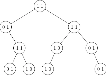
Fig. 3.1.Visualization of the binary tree from the Example in Sect. 3.2.1. 3. Our new space-efficient formats.

3.1. The arithmetical-coding-based (ACB) format. MatrixAcan be represented by a bit vectorB

of sizeM in whichN bits are set to 1 andM−N bits are set to 0. The probabilityp0that a given bit inB is

equal to 0 is M−N

M . In the arithmetical coding (see [21]), we can encode this information using −log2p0 bits.

The probability p1 that a given bit in B is equal to 1 is _MN. In the arithmetical coding, we can encode this

information using −log2p1 bits. Since we assume a random distribution of nonzero elements, the vector B is

considered to be an order-0 source (each bit is selected independently on other bits). The total number of bits to encode vectorB is equal to the value of binary entropy of vectorB. This value is

S(B) =−M·(p0log2p0+p1log2p1)

Since this expression is hard to compare with other formats, the approximation of the binary entropy of vector

B follows:

SACB(n, N) =−M ·(

M−N M log2

M −N M +

N M log2

N M)

=−(M−N) log2

M −N

M −Nlog2 N M

=−(M−N) log2(M −N) +Mlog2M −Nlog2N.

(5)

is then:

SACB(n, N)≈ N

ln 2 +Nlog2M −

N2

M·ln 2 −Nlog2N

≈N·

1

ln 2+ log2M−log2N

≈N·

1

ln 2+ 2·log2n−log2N

.

The same space complexity (based on other assumptions) was derived in [8], but it serves only for comparison and no practical algorithm to achieve this space complexity was given. As far as we know, the ACB format has not been described in literature.

The idea of transforming of the matrix A’s structure to the ACB format is simple: createn×n bitmap (with N 1’s) from matrix A’s structure. Then, compress this bitmap as a bitstream using the arithmetical coding. The representation of matrixA’s structure in the ACB format is given by the compressed bitstream.

A comparison to common SSFs is done in Sect. 5.2. A drawback of the ACB format is its computational complexity. Since each bit of vectorB is encoded in time Θ(1), the complete vectorB (representation of sparse matrixA) is encoded in time Θ(n2_{). This is too much for sparse matrices with a constant number of nonzero}

elements per row (i.e.,N ∈Θ(n)).

3.2. The minimal binary tree (MBT) format. The full binary tree (FBT) is a widely used data structure in which all inner nodes have exactly two child nodes. Binary trees especially those used for binary space partitioning can also be used for storing sparse matrices. The idea of binary space partitioning is not new, but as far as we know, the use of these formats for efficiently storing sparse matrices was not described in literature. In standard implementations, every node in a FBT is represented by a structurestandard_BT_struct consisting of the following items:

• two pointers (left,right) to child nodes,

• (only for leaves) the value of a nonzero element.

If a FBT is used as a basis for SSF, it describes a partition of the sparse matrix into submatrices and each node in the FBT represents a submatrix. Equally as in k-d trees, see [18], the decomposition is performed in alternating directions: first horizontally, then vertically, and so on. In other words, nodes in an odd height represent a partition of the submatrix into two halves along the the x-axis (left/right), nodes in an even height represent a partition of the submatrix into two halves along the y-axis (upper/lower). From the viewpoint of space efficiency, a drawback of the standard FBT representation is the overhead caused by pointersleft,right. It causes that the standard FBT-based SSF may have worse space complexity than the CSR format.

To eliminate this drawback, we propose a new k-d-tree-based SSF. Each tree node represents again a submatrix, but we modify the standard representation of the FBT and we call this data structure the minimal binary tree(MBT) format. The idea is very similar to that in the MQT format.

• All nodes of a MBT are stored in one array (or stream). Since the size of the input matrix is given, we can compute locations of all child nodes, we can omit pointersleft,right.

• All nodes of a MBT contain only two flags (it means only two bits). Each of them is set to 1 if the corresponding half of the submatrix (left/right or upper/lower) contains at least one nonzero element, otherwise it is set to 0.

A comparison of the MBT format with other SSFs is done in Sect. 5.3. Let us describe algorithm 2 that generates an output bitstream representing the matrix in the MBT format from the standard CSR format.

(6)

0 0

0

0 0 0

0

0 0 0

0 0

0

0 0 0

0

0 1 1

1 1

0

0 0 0

0

0 0 0

0 0

0

0 0 0

0

(a) Original sparse matrixA.

1 0

1 1

(b) The MBT representation of matrixA.

Fig. 3.2.The MBT with the minimal number of nodes.

h1

h2

1 1 ...

1 0

1 1 1 1

...

Fig. 3.3.MBT with the minimal number of nodes (the number of leaves isN/2).

shown in Fig. 3.1.

S= MBT(A) = MBT



  

0 0 0 1

0 0 1 0

1 0 0 0

0 0 0 1



  

=

= ”11” + MBT

0 0 0 1

0 0 1 0

+

+ MBT

1 0 0 0

0 0 0 1

=

= ”11” + ”01” + ”11” + MBT

0 1 1 0 + + MBT 1 0 0 0 + MBT 0 0 0 1 = = ”11” + ”01” + ”11” + ”11” + ”10” + ”01”+

+ MBT(”01”) + MBT(”10”) + MBT(”10”) + MBT(”01”) = = ”11” + ”01” + ”11” + ”11” + ”10”+

(7)

So, if matrix Ais stored in the MBT format, 20 bits are needed for representing its structure.

0 0

1

0 0 0

0

0 0 0

0 0

0

0 0 0

0

1

0

0 1 0

0 0

0

0 0 0

0

0 0 0

0 0

0

0 0 0

1

0

(a) Original sparse matrixA.

1 0

1 1

1 1 1 1

1 0 0 1 1 0 0 1 0 1 1 0 0 1 1 0 0 1 0 1 0 1 0 1

(b) The MBT representation of matrixA.

Fig. 3.4. The MBT with the maximal number of nodes.

h1

h2

1 1 ...

1 0 1 0

...

Fig. 3.5.MBT with the maximal number of nodes (the number of leaves isN/2).

3.2.2. Space complexity. Let us assume a very small example of a sparse matrix withn= 8 andN = 4. For common storage formats, the space complexity is given by Eq. (2.1) or (2.2), soSCOO(n, N) = 24[bits] and

SCSR(n, N) = 28[bits]. For the MQT, the exact size of the output bitstreamS (it means the size of the MBT

format) cannot be derived from these global parameters, because it depends on the exact locations of nonzero elements. It ranges from 14 to 38 bits (see Figs. 3.2 and 3.4). The derivation of the lower and upper bounds on the size of the MBT format in a general case is the following.

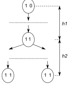
Lower bound. We consider the best case: the MBT with the minimal number of nodes, i.e., the number of leaves is equal to N/2 (see Fig. 3.3). It is obviously a generalized idea from Fig. 3.2. This matrix with 4 nonzero elements is represented by 7 MBT nodes = 14 bits. Output bitstream is ”10 10 10 10 11 11 11”.

• The height of the MBT on Fig. 3.2 is h = h1 +h2 = 2 log2n−1, where h2 = log2N −1 and

(8)

• All nodes with height< h1 (in upperh1 levels) contain exactly one 1 (they have one child node). The number of nodes in these levels is h1,

h1 = log2(n2/N).

• All nodes with height≥h1 (in lowerh2 levels) are full of 1’s (they have two child nodes). The number of nodes in these levels is equal to (this part is a full binary tree)

2 log2n−1 X

i=h1+1

2i−(h1+1)₌_N₋₁_.

So, the minimal size of the MBT format is

2· N−1 + log2(n2/N)

.

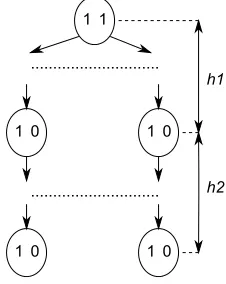
Upper bound. We consider the worst case: the quadtree with the maximal number of nodes, i.e., the number of leaves is equal toN/2 (see Fig. 3.5). Again, it is a generalized idea from Fig. 3.4. This matrix with 4 nonzero elements is represented by 19 MBT nodes = 38 bits.

The output bitstream is ”11 11 11 10 10 01 01 10 01 10 01 10 10 01 01 10 01 10 01”.

• The height of this tree ish=h1 +h2 = 2 log2n−1, whereh1 = log2N−1.

• All nodes with height< h1 (in upperh1 levels) are full of 1’s (they have two child nodes),h1 = log₂N−1. The number of nodes in these levels is approximately

h1−1

X

i=0

2i=N−1.

• All nodes with height ≥h1 (in lowerh2 levels) contain exactly one 1 (they have one child node). The number of nodes in these levels is

N·h2 =N·(2 log2n−log2N) =N·log2(n2/N).

So, the maximal size of the MBT format is

≈2·N 1 + log2(n2/N)

.

3.2.3. Time complexity of the transformation algorithm. Time complexity of the transforma-tion algorithm 2 is relatively high, because for each node in the MBT, it uses algorithm 1 with complexity

O(log2n·(y2−y1 + 1)). Fortunately, the average complexity is much lower (it depends on the value of the

parameteravg per row, distribution of nonzero elements, etc.).

We consider the worst case (similar ideas as for derivation of the space complexity in Sect. 3.2.2): the MBT with the maximal number of nodes, the number of leaves is equal to N (see Fig. 3.5). We assume that the time complexity of procedureAppendToBitstreamis Θ(1). ProcedureINES(A,x1,y1,x2,y2) is called for every node in the MBT in the output streamS two times.

• For nodes with height = h1: The number of these nodes is N, the expression (y2−y1 + 1) is equal to 1 +n/√N. Time complexity of the transformation for all nodes with this depth is Th1=N·(1 +

n/√N)·log2avg per row.

• For nodes with height =h1−1: The number of nodes isN/2 and the expression (y2−y1 + 1) is equal to 1 + 2n/√N. So, the total time complexity of the transformation for all nodes with depth≤h1 (in upperh1 levels) isTupper ≈Phi=01 Th1/2(i−h1)= Θ(N·(1 +n/

√

N)·log2avg per row).

• For nodes with height > h1: The time complexity of the transformation for all these nodes (for the lowerh2 levels) isTlower≈Phi=h1+1Th1/2(i−h1)= Θ(N(1 +n/

√

N)·log2avg per row).

So, the total time complexity of the transformation is

Θ(N(1 +n/√N)·log2avg per row).

(9)

Algorithm 1Procedure to test if the given submatrix is nonempty

1: procedureINES(A,x1,y1,x2,y2)

Input: A = an input submatrix in the CSR format

Input: x1,y1,x2,y2 = coordinates of the submatrix

Output: logical value indicating whether the given submatrix is nonempty

2: fory←y1, y2do

3: low←A.addr[y]; high←A.addr[y+ 1]

4: i←binary search(in array A.ci)

5: ⊲ within indexes fromhlow . . . highi

6: ⊲ to find a minimalisuch thatA.ci[i]≥x1

7: if C.ci[i]≤x2then

8: returntrue

9: end if

10: end for 11: returnf alse

12: end procedure

3.3. Compression of minimal formats. The MBT and MQT formats have minimal space complexity only if we assume fixed number of bits for each node (2 bits for MBT and 4 bits for MQT). We can relax this assumption to achieve more space efficient formats.

Lemma 3.1. Every node in the MBT (or in MQT) format (except for the root node for the zero matrixA) has got at least one bit equal to 1. The proof of Lemma 3.1 for the MBT format can be done by contradiction: if both bits in a MBT node X are zero, then this submatrix does not contain any nonzero element, so in the parent’s node of X the corresponding bit is set to 0 and node X is not included in the output stream and this is a contradiction with the initial assumption.

Similar proof can be done for the MQT format. Q.E.D.

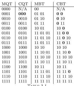
Since we assume only nonempty matrices, the only allowed values in every MBT node are: 01,10, and 11 (value 00 is not possible as a result of Lemma 3.1). So, if the first bit is 0, then the second bit must 1. This redundant information can be excluded from the output stream. We call this case thehidden one. Based on this idea, we propose a new format, calledcompressed binary tree (CBT). There are two approaches to transform a LSM to the CBT format:

1. Transform the input matrix to the MBT format (it creates output streamS) and then remove fromS

all hidden ones (all 4-tuples are read and transformed values according to Table 3.1 are written. 2. Modify Algorithm 2 to Algorithm 3 that directly create the CBT format.

(10)

Algorithm 2Transformation algorithm to the MBT format

1: procedureTr2MBT(A)

Input: A = the matrix for the transformation in CSR format

Output: S = the bitstream representing the input matrix in the MBT format

2: current←()

3: enqueue{1,1, A.n, A.n,0}into current

4: whilecurrentis not empty do

5: dequeue{x1, y1, x2, y2, h}fromcurrent

6: ⊲ x1,y1,x2,y2 = coordinates of submatrix

7: ⊲ h= current BFS level, divide rows (his odd) or columns

8: if his eventhen

9: mx←x2; my←(y1 +y2)/2 10: lx←x1; ly←(y1 +y2)/2 + 1

11: else

12: mx←(x1 +x2)/2; my ←y2

13: lx←(x1 +x2)/2 + 1; ly←y1

14: end if

15: l1←INES(A, x1, y1, mx, my)

16: l2←INES(A, lx, ly, x2, y2)

17: AppendToBitstream(S, l1)

19: if l1 =true then

20: enqueue{x1, y1, mx, my, h+ 1}into current

21: end if

23: enqueue{lx, ly, x2, y2, h+ 1}intocurrent 24: end if

25: end while 26: returnS

27: end procedure

3.3.1. An example of a transformation to the CBT format. For an example, we used the same matrix as in the example in Sect. 3.2.1. Hidden ones are denoted by bold numbers.

S= CBT(A) = CBT



  

0 0 0 1

0 0 1 0

1 0 0 0

0 0 0 1



  

=

= ”11” + CBT

0 0 0 1

0 0 1 0

+

+ CBT

1 0 0 0

0 0 0 1

=

= ”11” + ”0” + ”11” + CBT

0 1 1 0 + + CBT 1 0 0 0 + CBT 0 0 0 1 =

= ”11” + ”0” + ”11” + ”11” + ”10” + ”0”+

+ CBT(”01”) + CBT(”10”) + CBT(”10”) + CBT(”01”) = = ”11” + ”0” + ”11” + ”11” + ”10”+

(11)

Algorithm 3Transformation algorithm to the CBT format

1: procedureTr2CBT(A)

Input: A = the matrix for the transformation in CSR format

Output: S = the bitstream representing the input matrix in the CBT format

2: current←()

8: if his eventhen

9: mx←x2; my←(y1 +y2)/2 10: lx←x1; ly←(y1 +y2)/2 + 1

11: else

12: mx←(x1 +x2)/2; my ←y2

13: lx←(x1 +x2)/2 + 1; ly←y1

14: end if 15: l2←f alse

16: l1←INES(A, x1, y1, mx, my)

18: if l1 =truethen

19: l2←INES(A, lx, ly, x2, y2)

21: end if

23: enqueue{x1, y1, mx, my, h+ 1}into current 24: end if

26: enqueue{lx, ly, x2, y2, h+ 1}intocurrent

27: end if 28: end while 29: returnS

30: end procedure

(12)

MQT CQT MBT CBT

0000 N/A 00 N/A

0001 000 01 01 0 0 0010 0010 01 10 010 0011 0011 01 11 011 0100 0100 10 01 100 0101 0101 11 01 01 110 0 0110 0110 11 01 10 11010 0111 0111 11 01 11 11011 1000 1000 10 10 10 10 1001 1001 11 10 01 11 100 1010 1010 11 10 10 11 10 10 1011 1011 11 10 11 11 10 11 1100 1100 10 11 10 11 1101 1101 11 11 01 11 110 1110 1110 11 11 10 11 11 10 1111 1111 11 11 11 11 11 11

Table 3.1

(13)

Algorithm 4Transformation from the CBT format to the CSR format

1: procedureTr2CSR(S)

Input: S = the input bitstream of the input matrix in the CBT format

Output: A= the output matrix in the CSR format

2: A←newempty matrix

8: if x1 =x2 & y1 =y2 then

9: X ←newnonzero element (x1, y1)

10: addX toA

11: else

12: if his eventhen

13: mx←x2; my←(y1 +y2)/2

14: lx←x1; ly←(y1 +y2)/2 + 1

15: else

16: mx←(x1 +x2)/2; my←y2

17: lx←(x1 +x2)/2 + 1; ly←y1

18: end if

19: l1←ReadOneBit(S) 20: if l1 =f alsethen

21: l2←true ⊲ hidden one

22: else

23: l2←ReadOneBit(S)

24: end if

25: if l1 =truethen

26: enqueue{x1, y1, mx, my, h+ 1}intocurrent

27: end if

28: if l2 =truethen

29: enqueue{lx, ly, x2, y2, h+ 1}intocurrent

30: end if

31: end if 32: end while 33: returnA

(14)

4. Parallel execeution of transformation algorithm.

4.1. Main idea of parallelization. The proposed formats are generic, i.e., they may be applied to sparse matrices of any structure. When processing LSMs on a massively parallel computer system, every processor has its own part of a matrix, which itself can be treated as a stand-alone matrix of a smaller size. Every processor can apply one of the proposed formats to its own matrix independently. Hence, the proposed formats can be utilized on massively parallel computer systems the very same way as in sequential computations. This approach to parallelization is straightforward for the ACB format, but for SSFs based on trees the parallelization is more complicated.

Fig. 4.1.The main idea of parallelization of MBT or CBT transformation.

Fig. 4.2.The main idea of parallelization of MQT or CQT transformation.

4.2. Parallel transformation of formats based on trees. Consider the MBT format. The proposed Algorithm 2 for transformation is sequential. Let us now describe its master-slave parallelization. We assume two possible mappings how the matrix Ais distributed among processors:

• using general mapping.

• using row-wise 1D block mapping (see [17]). Matrix A is divided into P row blocks of variable size (recall P is the number of processors in a MPCS. This mapping uses array start row. In this array, the value start row[i] is the starting row for the row block assigned to processorpi.

The only difference is that for general mapping we must use a general (unoptimized) procedure ParINES

(15)

Algorithm 6).

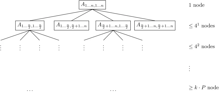
1. In the first step (Algorithm 8 and codelines 1-10 in Algorithm 7), only processor p1 (similarly to

Algorithm 2) expands nonempty nodes of a binary tree by BFS until the number of nodes (denoted by

C) is greater or equal tok·P, where k is the chosen constant (see Figs. 4.1 and 4.2, and Algorithm 7). The proper value of parameterkis the trade-off between better work-load balancing (higher values of k) and smaller sequential part of transformation (lower values ofk).

This binary tree defines partitioning of the matrix among processors. This tree (more exactly intervals of coordinates of nodes) is stored into arrayB and also stored in the MBT format in a special master file.

2. Initial communication (codeline 11 in Algorithm 7): Processorp1sends to all other processor blocks of

arrayB using one-to-all-scatter operation. The block forpi starts at index 1 + (i−1)⌈C/P⌉and ends at min(i⌈C/P⌉, C). Each block contains intervals of coordinates of submatrices that are assigned to the given processor (see Algorithm 6).

3. Redistribution of nonzero elements (codeline 12 in Algorithm 7): nonzero elements of the matrixAare redistributed between processors according to the resulting partitioning (arrayB).

4. Local transformation (codelines 13-20 in Algorithm 7): Every processor transforms assigned submatrices to the required MBT format independently and stores them into a separate file.

Algorithm 5Distributed procedure to test if the given submatrix is nonempty

1: procedureParINES(A,x1,y1,x2,y2)

Input: A = the input matrix in the distributed CSR format

Input: x1,y1,x2,y2 = coordinates of submatrix

2: one-to-all broadcast{x1, y1, x2, y2} 3: output=f alse

4: forj←y1, y2 do

5: fori←A.Addr[j], A.Addr[j+ 1]−1do 6: if (x1≥A.Ci[i]≤x2) then

7: output=true

8: break

9: end if

10: end for

11: end for

12: send predicateoutputto parallel reduction

13: po←parallel reduction ofoutputusing logical OR

14: returnpo

15: end procedure

Matrix n N avg per row

circuitM5 5.56·106

5.95·107

1.93·10−6

nlpkkt120 3.54·106

5.02·107

4.01·10−6

ldoor 9.52·105 _2.37_·₁₀7 _2.60_·₁₀−5

TSOPF RS b2383 3.81·104

1.62·107

1.10·10−2

mouse gene 4.51·104

1.45·107

7.10·10−3

t2em 9.25·105

4.59·106

5.36·10−6

bmw7st 1 1.41·105 _3.74_·₁₀6 _1.88_·₁₀−4

amazon0312 4.01·105

3.20·106

2.00·10−6

thread 2.97·104

2.25·106

2.55·10−3

gupta2 6.21·104 _2.16_·₁₀6 _5.60_·₁₀−4

c-29 5.03·103 _2.44_·₁₀4 _9.64_·₁₀−4

Table 4.1

(16)

Algorithm 6Distributed procedure to test if the given submatrix is nonempty

1: procedureParINES2(A,x1,y1,x2,y2)

Input: x1,y1,x2,y2 = coordinates of submatrix

2: constructG′

3: multicast{x1, y1, x2, y2}inG′

4: i←index of the current processor

5: si←start row[i]

6: si1←start row[i+ 1]

7: if (si > y2) OR (si1≤y1) then 8: output=f alse

9: else

10: fory←max(y1, si),min(y2, si1−1) do 11: low←A.addr[y]; high←A.addr[y+ 1]

12: i←binary search(in array A.ci)

13: ⊲ within indexes fromhlow . . . highi

14: ⊲ to find a minimalisuch thatA.ci[i]≥x1

15: if C.ci[i]≤x2 then 16: output=true

17: break

18: end if

19: end for

20: output=f alse 21: end if

22: send predicateoutputto parallel reduction

23: po←parallel reduction ofoutputusing logical OR inG′ 24: returnpo

25: end procedure

5. Results of space efficient formats.

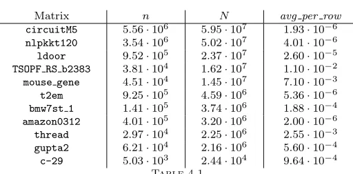
5.1. Testing matrices. We have used 11 testing matrices from various application domains from the University of Florida Sparse Matrix Collection [5]. Table 4.1 shows the characteristics of the testing matrices. For quantification of the reduction in data-representation size produced by a data format, we have used ratio of space complexities. For comparison of the results, we have used these common formats:

• the COO format,

• the CSR format,

• the text-based Matrix Market format [4],

• the zipped Matrix Market format (we have used the PKZIP program with the option for maximal compression).

For our purposes, we have excluded all temporary informations from the source Matrix Market files (like comments and values of nonzero values).

5.2. Comparison of space complexities of common and ACB SSFs. Table 5.1 illustrates the fact that the space complexity of storing the structure of these sparse matrices using common storage formats (COO and CSR) are significantly greater than in the ACB format (independently on the padding). We can conclude that the common SSFs (COO, CSR) are not suitable for our purposes.

(17)

Algorithm 7Parallel transformation algorithm to the MBT format

1: procedureParTr2MBT(A)

Output: S = the local bitstream of the resulting MBT format

2: i←index of the current processor

3: if i= 1then ⊲master section

4: S←()

5: enqueue{A,1,1, A.n, A.n,0}intocurrent

6: while|current|< k·P do

7: current ←ExpandLevel(S,current) 8: end while

9: storeS in master file 10: convertcurrent to arrayB

11: end if 12: barrier

13: one-to-all scatter of B

14: all-to-all scatter of matrix structure

15: S←()

16: C← |current|

17: forj←1 + (i−1)⌈C/P⌉,min(i⌈C/P⌉, C)do 18: _{x1, y1, x2, y2, h} ←B[j]

19: D←A[y1. . . y2][x1. . . x2]

20: Tr2MBT(D, x1, y1, x2, y2, h)

21: end for

22: storeS in separate file dedicated topi

23: return 24: end procedure

Matrix COO COO CSR CSR

SMIN _SPOW _SMIN _SPOW

circuitM5 2.25 3.13 1.24 1.71

nlpkkt120 2.27 3.30 1.23 1.77

ldoor 2.40 3.84 1.26 2.00

TSOPF RS b2383 4.04 4.04 2.03 2.03

mouse gene 3.73 3.73 1.87 1.88

t2em 2.11 3.38 1.30 2.03

bmw7st 1 2.61 4.63 1.36 2.40

amazon0312 2.23 3.75 1.28 2.11

thread 2.98 3.18 1.52 1.63

gupta2 2.61 2.61 1.36 1.38

c-29 2.27 2.79 1.40 1.68

Table 5.1

The ratio of the space complexities of matrices in the COO or CSR formats using different paddings and in the ACB format.

other storage schemes. CR stands forcompression rate. CR1 denotes the ratio of the MBT to the (CSR,SPOW) format space complexities. CR2 denotes the ratio of the MBT to the ACB format space complexities. CR3 denotes the ratio of the MBT format space complexity to space complexity of the text based Matrix Market format. CR4 denotes the ratio of the MBT format space complexities to the zipped Matrix Market format space complexity.

Table 5.3 shows ratios of space complexities of the four tree-based formats studied in this paper to the ACB format. From this table, we can observe that the CBT format:

(18)

Algorithm 8Master section of parallel transformation algorithm to the MBT format

1: procedureExpandLevel(S,current)

2: create empty queue new

3: whilecurrent is nonemptydo

5: if his eventhen

6: mx←x2; my←(y1 +y2)/2

7: lx←x1; ly←(y1 +y2)/2 + 1

8: else

9: mx←(x1 +x2)/2; my ←y2 10: lx←(x1 +x2)/2 + 1; ly←y1 11: end if

12: l1←ParINES(A, x1, y1, mx, my)

13: l2←ParINES(A, lx, ly, x2, y2)

17: enqueue{A, x1, y1, mx, my, h+ 1}into next

18: end if

20: enqueue{A, lx, ly, x2, y2, h+ 1} intonext

21: end if 22: end while 23: returnnext 24: end procedure

Matrix CR1 [%] CR2 [%] CR3 [%] CR4 [%]

circuitM5 16.5 28.3 4.9 28.8

nlpkkt120 12.8 22.6 3.5 25.6

ldoor 8 16.1 2.4 15.3

TSOPF RS b2383 15.6 31.5 2.7 14.0

mouse gene 73.0 137.0 12.8 53.9

t2em 16.3 33.0 5.7 26.2

bmw7st 1 8.5 20.3 2.8 15.7

amazon0312 53.1 112.1 18.1 67.7

thread 16.4 26.8 3.0 14.4

gupta2 28.7 39.7 5.3 23.3

c-29 31.7 53.4 8.6 27.2

Table 5.2

Comparison of the space complexity of the MBT format with that of other storage schemes.

• has similar space complexity as the MQT or CQT formats. We can conclude that the CBT format is very space efficient.

5.4. Results for parallelization of the tree-based formats. The most time-consuming part of master section of ParTr2MBTprocedure (parallel implementation of conversion to the MBT format) is the blocking call of ParINES(or ParINES2) procedure. To achieve good scalability of this code, the overhead of these calls should be small in comparison to the global parameters (nandN), because these parameters influence the time complexity of parallel section (local transformation) of ParTr2MBTprocedure (see Sect. 3.2.3).

(19)

Matrix MBT [%] CBT [%] MQT [%] CQT [%]

circuitM5 27,4 24,4 26,6 26,5

nlpkkt120 26,1 23,5 19,8 19,8

ldoor 22,5 21,2 14,4 14,3

TSOPF RS b2383 36,1 35,9 33,6 33,5

mouse gene 130,8 111,0 130,4 128,0

t2em 36,6 31,7 29,9 29,4

bmw7st 1 26,3 25,0 20,3 20,3

amazon0312 110,8 89,1 107,1 103,1

thread 37,3 35,3 23,8 23,8

gupta2 48,0 42,3 36,3 36,0

c-29 55,7 48,8 51,3 50,9

Table 5.3

Comparison of the space complexity of the tree-based SSFs with that of the ACB format.

Matrix n N #calls (kP = 101

) #calls (kP= 102

) #calls (kP = 103

)

circuitM5 5.56·106

5.95·107

20 278 4248

nlpkkt120 3.54·106

5.02·107

26 452 3852

ldoor 9.52·105

2.37·107

26 240 2204

TSOPF RS b2383 3.81·104 _1.62_·₁₀7 ₂₀ ₃₇₈ ₃₂₁₀

mouse gene 4.51·104

1.45·107

22 220 2060

t2em 9.25·105

4.59·106

26 426 4906

bmw7st 1 1.41·105 _3.74_·₁₀6 ₂₂ ₂₃₂ ₃₃₆₈

amazon0312 4.01·105 _3.20_·₁₀6 ₁₈ ₂₀₀ ₂₀₇₂

thread 2.97·104 _2.25_·₁₀6 ₂₆ ₂₆₀ ₃₄₈₆

gupta2 6.21·104

2.16·106

28 380 3888

c-29 5.03·103

2.44·104

26 348 3900

Table 5.4

The efficiency of parallel algorithm (the number of calls of ParINES).

6. Conclusions. This paper deals with the design of four new SSFs called arithmetical coding based format, minimal binary tree format, compressed binary tree format, and compressed quadtree format. These formats have been designed in order to minimize the space complexity. We performed experiments with these formats and compared them with other common SSFs (COO or CSR) and other schemes used for LSMs in a file. These experiments proved that our new formats can significantly reduce the amount of data needed for storing LSMs. We have also presented a parallel algorithm for transformation of a LSM in the CSR format to one of these newly proposed formats.

REFERENCES

[1] T. Dytrych, K. D. Launey, J. P. Draayer, P. Maris, J. P. Vary, E. Saule, U. Catalyurek, M. Sosonkina, D. Langr, and M. A. Caprio, Collective Modes in Light Nuclei from First Principles, PHYSICAL REVIEW LETTERS, 111 (2013).

[2] K. D. Launey, S. Sarbadhicary, T. Dytrych, and J. P. Draayer,Program in C for studying characteristic properties of two-body interactions in the framework of spectral distribution theory, COMPUTER PHYSICS COMMUNICATIONS, 185 (2014), pp. 254–267.

[3] R. Barrett, M. Berry, T. F. Chan, J. Demmel, J. Donato, J. Dongarra, V. Eijkhout, R. Pozo, C. Romine, and H. V. der Vorst,Templates for the Solution of Linear Systems: Building Blocks for Iterative Methods, SIAM, Philadelphia, PA, 2nd ed., 1994.

[4] R. F. Boisvert, R. Pozo, and K. Remington,The Matrix Market Exchange Formats: Initial Design, Tech. Report NISTIR 5935, National Institute of Standards and Technology, Dec. 1996.

[5] T. A. Davis,The university of florida sparse matrix collection, NA DIGEST, 92 (1994).

[6] E. Im,Optimizing the Performance of Sparse Matrix-Vector Multiplication - dissertation thesis, Dissertation thesis, University of Carolina at Berkeley, 2001.

[7] I. ˇSimeˇcek, D. Langr, and P. Tvrdik, Minimal quadtree format for compression of sparse matrices storage, in 14th International Symposium on Symbolic and Numeric Algorithms for Scientific Computing (SYNASC’2012), SYNASC’2012, Timisoara, Romania, sept. 2012, pp. 359–364.

(20)

Systems (HPCC-ICESS), HPCC’12, Liverpool, Great Britain, june 2012, pp. 54–60.

[9] I. ˇSimeˇcek, D. Langr, and P. Tvrd´ık,Space efficient formats for structure of sparse matrices based on tree structures, in Proceedings of 15th International Symposium on Symbolic and Numeric Algorithms for Scientific Computing (SYNASC 2013), SYNASC ’13, 2013. to be published.

[10] I. ˇSimeˇcek and P. Tvrd´ık,Sparse matrix-vector multiplication - final solution?, in Parallel Processing and Applied Mathe-matics, vol. 4967 of PPAM’07, Berlin, Heidelberg, 2008, Springer-Verlag, pp. 156–165.

[11] D. Langr, I. ˇSimeˇcek, P. Tvrd´ık, T. Dytrych, and J. P. Draayer,Adaptive-blocking hierarchical storage format for sparse matrices, in Federated Conference on Computer Science and Information Systems (FedCSIS), 345 E 47TH ST, NEW YORK, NY 10017 USA, September 2012, IEEE Xplore Digital Library, pp. 545–551.

[12] D. Langr, I. ˇSimeˇcek, and P. Tvrd´ık,Storing Sparse Matrices in the Adaptive-Blocking Hierarchical Storage Format, in Federated Conference on Computer Science and Information Systems (FedCSIS), September 2013, IEEE Xplore Digital Library, pp. 479–486.

[13] M. Martone, S. Filippone, M. Paprzycki, and S. Tucci, On the usage of 16 bit indices in recursively stored sparse matrices, in Proceedings of the 2010 12th International Symposium on Symbolic and Numeric Algorithms for Scientific Computing, SYNASC ’10, Washington, DC, USA, 2010, IEEE Computer Society, pp. 57–64.

[14] M. Martone, S. Filippone, S. Tucci, P. Gepner, and M. Paprzycki,Use of hybrid recursive csr/coo data structures in sparse matrix-vector multiplication, in Computer Science and Information Technology (IMCSIT), Proceedings of the 2010 International Multiconference on, Oct 2010, pp. 327–335.

[15] M. Martone, S. Filippone, S. Tucci, and M. Paprzycki, Assembling recursively stored sparse matrices, in Computer Science and Information Technology (IMCSIT), Proceedings of the 2010 International Multiconference on, Oct 2010, pp. 317–325.

[16] M. Martone, M. Paprzycki, and S. Filippone,An improved sparse matrix-vector multiply based on recursive sparse blocks layout, in Large-Scale Scientific Computing, vol. 7116 of Lecture Notes in Computer Science, Springer Berlin Heidelberg, 2012, pp. 606–613.

[17] A. Pinar and C. Aykanat,Sparse matrix decomposition with optimal load balancing, in Proceedings of the Fourth Inter-national Conference on High-Performance Computing, HIPC ’97, Washington, DC, USA, 1997, IEEE Computer Society, pp. 224–.

[18] L. Romero and E. Zapata,Data distributions for sparse matrix vector multiplication, Parallel Computing, 21 (1995), pp. 583 – 605.

[19] Y. Saad,Iterative Methods for Sparse Linear Systems, Society for Industrial and Applied Mathematics, Philadelphia, PA, USA, 2nd ed., 2003.

[20] P. Tvrd´ık and I. ˇSimeˇcek,A new diagonal blocking format and model of cache behavior for sparse matrices, in Proceedings of the 6th International Conference on Parallel Processing and Applied Mathematics, vol. 12 of PPAM’05, Poznan, Poland, 2005, Springer-Verlag, pp. 164–171.

[21] I. H. Witten, R. M. Neal, and J. G. Cleary,Arithmetic coding for data compression, Commun. ACM, 30 (1987), pp. 520– 540.

[22] M. Tuma,Overview of direct methods, I. Winter School of SEMINAR ON NUMERICAL ANALYSIS, January 2004, Ostrava, Czech Republic.

Edited by: Teodor Florin Forti¸s Received: Mar 3, 2014