A simulation study on matched case-control designs in the perspective of causal diagrams

(1)

R E S E A R C H A R T I C L E

Open Access

A simulation study on matched

case-control designs in the perspective

of causal diagrams

Hongkai Li, Zhongshang Yuan, Ping Su, Tingting Wang, Yuanyuan Yu, Xiaoru Sun and Fuzhong Xue

*

Abstract

Background:In observational studies, matched case-control designs are routinely conducted to improve study precision. How to select covariates for match or adjustment, however, is still a great challenge for estimating causal effect between the exposure E and outcome D.

Methods:From the perspective of causal diagrams, 9 scenarios of causal relationships among exposure (E), outcome (D) and their related covariates (C) were investigated. Further various simulation strategies were

performed to explore whether match or adjustment should be adopted. The“do calculus”and“back-door criterion” were used to calculate the true causal effect (β) of E on D on the log-odds ratio scale. 1:1 matching method was used to create matched case-control data, and the conditional or unconditional logistic regression was utilized to get the estimators (⌢β) of causal effect. The bias (⌢β‐β) and standard error (SEð⌢βÞ) were used to evaluate their performances.

Results:When C is exactly a confounder for E and D, matching on it did not illustrate distinct improvement in the precision; the benefit of match was to greatly reduce the bias forβthough failed to completely remove the bias; further adjustment for C in matched case-control designs is still essential. When C is associated with E or D, but not a confounder, including an independent cause of D, a cause of E but has no direct causal effect on D, a collider of E and D, an effect of exposure E, a mediator of causal path from E to D, arbitrary match or adjustment of this kind of plausible confounders C will create unexpected bias. When C is not a confounder but an effect of D, match or adjustment is unnecessary. Specifically, when C is an instrumental variable, match or adjustment could not reduce the bias due to existence of unobserved confounders U.

Conclusions:Arbitrary match or adjustment of the plausible confounder C is very dangerous before figuring out the possible causal relationships among E, D and their related covariates.

Keywords:Simulation study, Matched case-control designs, Causal diagrams

Background

In observational studies, confounding factors (C) that are pre-exposure variables associated with the exposure E and the outcome D will distort the estimation of the

target causal effect [1–4]. Generally, the magnitude of

confounding bias mainly depends on the strength of the effects from confounder C to exposure E and from con-founder C to outcome D. If one of these two effects is precisely null, confounding bias does not exist at all.

Furthermore, the directions of effect from C to E and from C to D determine the direction of the bias. Usually, confounding factors could mainly lead to three kinds of biases in an attempt to find the causal effect from E to D, including over-estimation, under-estimation, or even missing the direction of the effect [5].

In analytic epidemiology, various strategies could be adopted to remove confounding bias, such as Restric-tion, Adjustment, Stratification [6, 7], while strategy of matching on confounders C (e.g. matched case-control designs) mainly focuses on improving estimation preci-sion of the effect of E on D, rather than removing * Correspondence:[email protected]

Department of Biostatistics, School of Public Health, Shandong University, Jinan City, Shandong Province, People’s Republic of China

(2)

confounding bias [8, 9]. For matched case-control de-signs, matching refers to the selection of controls group that is identical, or nearly so, to the cases group with re-spect to the distribution of one or more potentially con-founding factors. Generally, two matching strategies, including individual matching and frequency matching, could be selected to force the distribution of the match-ing factors to be identical across groups of individuals [10]. In particular, individual matching involves selection of one or more controls group with matching factor values equal to cases group. From the perspective of causal diagrams, several qualitative studies had suggested that matching on confounders not only fails to remove

confounding bias but also adds colliding bias [11–15].

Therefore, it is still necessary to adjust for the matching variables.

However, for obtaining unbiased and precise estima-tion, it is crucial to choose matching variables cor-rectly and further determine whether they should be adjusted for. For matching variables, matching on common child nodes of exposure and outcome, or me-diators of the exposure and outcome will generally lead to irremediable bias [13, 14]. For further adjustment, conditional logistic regression models are customarily

used to adjust for matching variables, which just pro-vide conditional rather than causal estimation of odds ratio [16]. Sometimes, unconditional logistic regres-sion models can also be adopted to adjust for match-ing variables, but they will lead to lower precision for the parameters estimation when the number of matched variables is larger under given limited sample size [17].

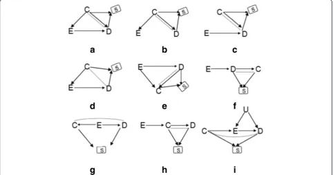
In this paper, we performed various quantitative simu-lations under the following 9 scenarios to illustrate the benefits of correct match and further proper adjustment, and to highlight the consequences of improper match and further inappropriate adjustment. a) C is a con-founder for the exposure E and the outcome D (Fig. 1a); b) C is a common cause of E and D with an absence of cause effect between them (Fig. 1b); c) C is an independ-ent cause of D (Fig. 1c); d) C is a cause of E, but has no direct causal effect on D (Fig. 1d); e) C is a common ef-fect (i.e. collider) of E and D (Fig. 1e); f ) C is an efef-fect of outcome D (Fig. 1f ); g) C is an effect of exposure E (Fig. 1g); h) C is a mediator of causal path from E to D (Fig. 1h); i) C is an instrumental variable for E and D (Fig. 1i). All above scenarios almost involve common roles of C in analytic epidemiology.

(3)

Methods

A brief introduction to causal diagrams and calculation of causal effect

In the past few decades, causal diagrams, one kind of di-rected acyclic graphs (DAGs), have been widely used to visually summarize hypothetical causal relations among variables of interest. Modern causal diagrams were more recently developed to merger probability theory with

path diagrams [2, 18–20]. The resulting theory provides

a powerful yet intuitive device for deducing the statis-tical associations implied by causal relations. Further-more, given a set of observed statistical associations, a researcher armed with causal diagrams theory can sys-tematically characterize all causal analysis. In causal

dia-grams, the d-Separationcriterion is an essential graphic

rule for linking causal relations to statistical associations [20, 21]. They help epidemiologists to draw logically sound conclusions about certain types of statistical rela-tions and facilitate many tasks, such as understanding confounding bias and selection bias [15], choosing co-variates for adjustment or match [10], analyzing direct and indirect effects [22], using instrumental variable to estimate causal effect when unobserved confounders exist [23]. In this paper, we used causal diagrams to illustrate the relationships among variables in above 9 scenarios.

Furthermore,do-calculustogether withback-door

criter-ionproposed by Pearl [20, 24, 25] were used to calculate

the causal effect of exposure (X) on outcome (Y). Given a

causal diagramG, together with non-experimental data on

a subset V of observed variables in G, we estimate the

causal effect of X on Y by calculatingP(y|do(X=x)) from

a sample estimation ofP(V =v). Namely, we aim to

esti-mate what the interventiondo(X = x) would have on a set

of response variable Y, whereX andYare two subsets of

V. For identifyingP(y|do(X=x)), the“back-door criterion”

[20] was further used to test if a setZ⊆Vof variables is

sufficient, where Z satisfied the following conditions. (i) it blocked every path from X to Y that has an arrow into

X (“blocks the back door”); and (ii) no node in Z is a

descendant of X. If a set of variable Z satisfies the back-door criterion relative to (X, Y), then the causal effect of X on Y is identifiable and is calculated by the following formula,

P yð jdo Xð ¼xÞÞ ¼X

Z

P yð jx;zÞP zð Þ

In this paper, this formula was used to calculate the

true causal effect β of exposure E on outcome D from

source population. It was regarded as a gold standard to assess the bias of estimation in all 9 simulation scenarios.

Simulation scenarios

Figure 1 showed the causal diagrams of 9 simulation sce-narios for estimating causal effect of E on D, which illus-trated 9 different roles of C respectively. Based on Fig. 1(a) to (i), Monte Carlo simulations were used to generate simu-lation data. We made the following assumptions for the simulation: 1) all variables are binary following a Bernoulli distribution; 2) the correlations between variables are positive unless otherwise specified; and 3) the associ-ation between covariates (E and C) and the outcome D is log-linearly additive effect. Logistic regression models were used to simulate child nodes from their correspond-ing parent nodes. Take scenario 1 [seecorrespond-ing Fig. 1(a)] as an

example, letP(C= 1) =π,thenP(E= 1|C) = exp(α0+α1C)/

[1 + exp(α0+α1C)] for the child node E from its parent

node C; similarly,P(D= 1|C,E) = exp(β0+β1C+β2E)/[1 +

exp(β0+β1C+β2E)]; where the parametersα0,β0denoted

the baseline prevalence of E and D respectively, and each

ef-fect parameter (α1,β1,β2) refers to the log-odds ratio

condi-tional on other covariates. The simulated source population with 100,000 subjects was generated from above procedure. 1000 cases were randomly sampled from this simulated source population with D = 1, while 1000 controls were ran-domly sampled from D = 0; so far none-matched case-control data with 1000 cases and 1000 case-controls was created. For matched case-control data, we still used the above same 1000 cases as the cases group, for individual with C = 1 in cases group, we matched its control by randomly sampling a subject with C = 1 and D = 0 from the source population; similarly, for individual with C = 0, we matched its control with C = 0 and D = 0 from the source population.

Besides, unconditional and conditional regression models were applied to above two datasets to assess their perfor-mances. For non-matched case-control data, both uncondi-tional logistic regression model without adjusting for C, logit p Dð ð ¼1jEÞÞ ¼β₀þβ′₁E, (model 1), and with

adjust-ing for C, logit(p(D= 1|E,C)) =β0+β1″E +β2C, (model 2),

were performed for comparing their bias (⌢β₁‐β, where⌢β₁

was the estimation by the logistic regression models, while

β was the true causal effect from source population) and

precision by the standard error of⌢β₁(SEðβ⌢₁Þ). For matched

case-control data, the following three models were used to

compare their bias (⌢β₁‐β) and precision (SEðβ⌢₁Þ): model 3)

unconditional logistic regression without adjusting for C; model 4) unconditional logistic regression with adjusting for C; and model 5) conditional logistic regression.

Various simulation scenarios were performed by varying

across a target effect parameter [e.g. C→E in Fig. 1(a)]

and keeping all others constant to explore the trends of

bias (⌢β₁‐β) and standard error (SEðβ⌢₁Þ). 1000 simulations

(4)

Results

Scenario 1 (C is a confounder for E and D, Fig. 1a)

Theoretically, in this scenario, the confounder C is

d-connectedwith outcome D via two natural paths: C→D

and C→E→D, which contribute to the crude association

between C and D. Nevertheless, under matched case-control designs, C is unconditionally independent of D due to the identical distribution of C in cases and controls

group (i.e. the sum of C→D, C→E→D and C–D is null).

Furthermore, the path C–D is of equal magnitude, but

op-posite direction to the C→E→D and C→D. Therefore,

the joint distribution of E, C and D is unfaithful to the DAG of Fig. 1a due to matching on C. As C is a confounder, both

paths C→E and C→D will lead to the bias for E on D

before matching, while after matching, a new colliding

bias path C–D is created and the two bias paths (C→E,

C→D) still exist. In this situation, the total bias is

con-tributed by the path of C→E, C→D and C–D [13–15].

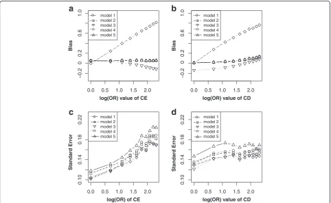
Figure 2 showed the simulation results under scenario 1. It indicated that given other parameters fixed and

varying across the effect of C→E (Fig. 2a), the bias (⌢β₁‐β)

elevated linearly with effects of C→E increasing in the

model without adjusting for C under non-matched case-control designs (model 1), while elevated in the opposite

direction with effects of C→E increasing in the model

without adjusting for C under matched case-control de-signs (model 3); after adjusting for C, the bias was ap-proximate to zero in all models of adjustment for C under non-matched case-control designs (model 2) and matched case-control designs (model 4 or model 5). For their

preci-sion (Fig. 2c), the SEðβ⌢₁Þ of all above five models

in-creased with effects of C→E increasing, and model 5

obtained largest standard error, followed by model 4, model 2, model 3, model 1. Similarly, given other

pa-rameters fixed and varying across C→D (Fig. 2b), the

bias (⌢β₁‐β) still elevated linearly with effects of C→D

increasing in model 1, while lowered with effects of

C→D increasing in model 3. After adjusting for C, the

bias was still nearly approximate to zero in model 2,

model 4 or model 5. For their precision (Fig. 2d), theS

Eðβ⌢1Þ of all above five models kept stable with effects

of C→D increasing, and model 5 attained largest standard

0.0 0.5 1.0 1.5 2.0

−0.2

0.2

0.6

1.0

log(OR) value of CE

Bias

model 1 model 2 model 3 model 4 model 5

0.0 0.5 1.0 1.5 2.0

−0.2

0.2

0.6

1.0

log(OR) value of CD

Bias

0.0 0.5 1.0 1.5 2.0

0.10

0.14

0.18

0.22

log(OR) of CE model 1

model 2 model 3 model 4 model 5

0.0 0.5 1.0 1.5 2.0

0.10

0.14

0.18

0.22

log(OR) value of CD model 1

StandaStandard Error

0 0

Standard Error

(5)

error, followed by model 4, model 2, model 1, model 3. These results suggested that confounding bias and colliding bias generally changed in opposite directions and adjust-ment was indispensable after matching on C.

Scenario 2 (C is a common cause of exposure E and outcome D without causal effect between them, Fig. 1b) It is similar to scenario 1 (Fig. 1a) except that instead of having causal effect between E and D. In this situation,

the path C→D leads to the association of C and D in a

non-matched case-control designs. But two effect paths of C and D offset each other after matching, that is the

effect of C–D is of equal magnitude, but opposite

direc-tion to C→D [14].

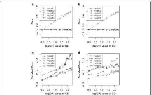
Simulation showed that (Fig. 3): keeping other

parame-ters constant, and varying across C→E (Fig. 3a), the

bias (⌢β₁‐β) elevated linearly with effects of C→E

in-creasing in the model without adjusting for C under non-matched case-control designs (model 1), while ap-proximate unbiased estimations were got in model 2, model 3, model 4 and model 5. All five models revealed

an increased effect with effects of C→E increasing.

Among them, model 2 got largest standard error, followed by model 4, model 5, model 3 and model 1.

Similarly, as E←C→D is a confounding path (Fig. 3b),

the bias (⌢β₁‐β) elevated linearly with effects of C→D

increasing in model 1, while the bias was almost null after adjustment (model 2, model 3, model 5) or match

(model 4). The SEðβ⌢₁Þ revealed a linearly increasing

trend for the five models, while the model 2 illustrated largest standard error, followed by model 4, model 5, model 1, model 3. These results indicated that both matching and adjustment could block the bias path

E←C→D, but adjustment for C would lead to lower

precision. Therefore, the best choice is the model with-out adjusting for C in matched case-control designs (model 3) in scenario 2.

Scenario 3 (C is a cause of outcome D, Fig. 1c)

As C is not a confounder, C and E are independent causes of D, respectively, the marginal effect from E to

0.0 0.5 1.0 1.5 2.0

−0.2

0.2

0.6

1.0

Bias

0.0 0.5 1.0 1.5 2.0

−0.2

0.2

0.6

1.0

Bias

0.0 0.5 1.0 1.5 2.0

0.08

0.10

0.12

0.0 0.5 1.0 1.5 2.0

0.08

0.10

0.12

StandaStandard Error

0 0

Standard Error

Fig. 3Bias (upper panels) and standard error (i.e. SE,lower panels) of log transformed odds ratio estimations for different effect sizes of CE and CD. Eachlineindicated one model. Theleft paneldisplayed the bias and standard error of different odds ratio (from 1 to 10) of CE. Theright panel

(6)

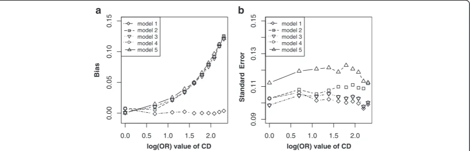
D is an unbiased estimator. In this situation, matching on or adjustment for C will inevitably lead to bias for E on D due to conditional on C by matched case-control designs or logistic regression model [14].

As expected, only model without adjusting for C in non-matched case-control designs (model 1) got un-biased and precise estimation (Fig. 4), and both match and adjustment would increase bias and lower precision

with effects of C→D increasing in model 2 to model 5.

Scenario 4 (C is a cause of exposure E, Fig. 1d)

The C has a direct effect on E and an indirect effect on D through E. So C is not a confounder for E and D. In this situation, if matching on C, a new association is

generated between C and D (denoted with C–D). Thus

E←C–D becomes an open bias path for E on D [14].

Simulation results (Fig. 5) supported above deductions, and revealed that only model without adjusting for C in matched case-control designs (model 3) led to bias (Fig. 5a). In matched case-control designs, although the bias could be remedied by adjusting for C, the precision (Fig. 5b) would become lower (model 4 and model 5).

Scenario 5 (C is a common effect of exposure E and outcome D, Fig. 1e)

In this scenario, as C is not a confounder but a collider, match on or adjustment for C (model 2 to model 5) will generate colliding bias [14, 15]. The simulation results

under varying across the effects of E→C and C←D

(Fig. 6) verified that only model without adjusting for C in non-matched case-control designs (model 1) got un-biased estimation.

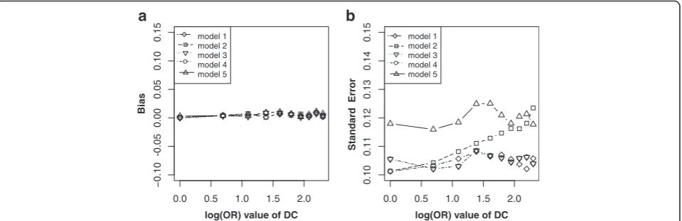
Scenario 6 (C is an effect of outcome D, Fig. 1f)

In this scenario, the C is not a confounder but an effect (child node) of outcome D, so match on or adjustment for C is not necessary. Simulation results showed that both matching on C and adjusting for C did not lead to

bias ofβ(Fig. 7a), but adjustment for C (model 2, model

4 and model 5) led to lower precision (Fig. 7b).

Scenario 7 (C is an effect of exposure E, Fig. 1g)

For this scenario, although C is associated with E (E→C)

and D (C←E→D), it is not a confounder. In practice, it

is difficult to distinguish it from confounder by statistical association study. Theoretically, matching on this kind of

spurious confounders will open bias path E→C–D and

thus lead to biased estimation ofβ. On the other hand,

ad-justment for C will not lead to biased estimation ofβbut

will lower its precision. Simulation results are concordant with above deductions, which revealed the biased

estima-tion of β (Fig. 8a) by matching on C (model 3), and

showed lower precision (Fig. 8b) by adjusting for C (model 2, model 4 and model 5).

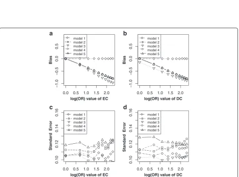
Scenario 8 (C is a mediator of causal path from E to D, Fig. 1h)

In this scenario, although C is associated with E (E→C)

and D (C→D), it is not a confounder but a mediator.

Matching on C will block the path E→C, while

adjust-ing for C will block the path C→D. Therefore, either

match or adjustment will inevitably block the causal

path E→C→D, and thus leads to the biased estimation

ofβ[14]. Both Fig. 9a and b illustrated that only model

without adjusting for C in non-matched case-control

de-signs (model 1) got unbiased estimation of β in the

Bias

0.0 0.5 1.0 1.5 2.0

0.00

0.05

0.10

0.15 model 1 model 2 model 3 model 4 model 5

0.0 0.5 1.0 1.5 2.0

0.09

0.11

0.13

0.15

log(OR) value of CD model 1

Standard

Error

Fig. 4Bias (left panels) and standard error (i.e. SE,right panels) of log transformed odds ratio estimations for different effect sizes of CD. Eachline

(7)

0.0 0.5 1.0 1.5 2.0

−0.2

0.0

0.1

0.2

0.3

Bias

0.0 0.5 1.0 1.5 2.0

0.10

0.12

0.14

0.16

0.18

0.20

log(OR) value of CE model 1

Standard

Error

Fig. 5Bias (left panels) and standard error (i.e. SE,right panels) of log transformed odds ratio estimations for different effect sizes of CE. Each line represented one model.Note: model 1, unconditional logistic regression model without adjusting for C for non-matched case-control designs; model 2, unconditional logistic regression model with adjusting for C for non-matched case-control designs; model 3, unconditional logistic regression model without adjusting for C for matched case-control designs; model 4, unconditional logistic regression model with adjusting for C for matched case-control designs; model 5, conditional logistic regression model with adjusting for C for matched case-control designs

0.0 0.5 1.0 1.5 2.0

−1.0

−0.5

0.0

0.5

log(OR) value of EC

Bias

0.0 0.5 1.0 1.5 2.0

−1.0

−0.5

0.0

0.5

log(OR) value of DC

Bias

0.0 0.5 1.0 1.5 2.0

0.10

0.12

0.14

0.16

0.0 0.5 1.0 1.5 2.0

0.10

0.12

0.14

0.16

Standard

Error

Standard

Error

(8)

situation of varying across effects of E→C and C→D.

In these two situations, lower precision of ⌢β₁ (Fig. 9c

and d) were observed by adjusting for C (model 2, model 4 and model 5).

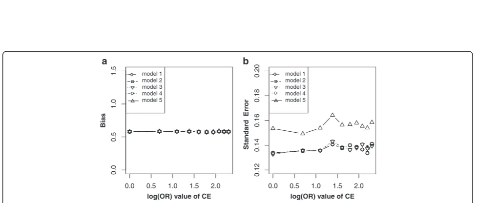
Scenario 9 (C is an instrumental variable for E and D, Fig. 1i)

In Fig. 10, we can easily find that C is not a confounder but an instrumental variable (IV), though C is associated

with E (C→E) and D (C→E→D). This instrumental

variable C can be used to control for the unobserved confounder U for estimating the causal effect of E on D [26]. However, instead of controlling for the confounding effect of U through either matching on or adjusting for C,

the biased estimation for effect of E→D could not be

reduced. The simulation results (Fig. 10) indicated that all the five models led to similar bias.

Discussion

From the perspective of causal diagrams, several studies had claimed that matching on confounders C in matched case-control designs can improve estimation precision for the effect of exposure (E) on outcome (D), though it fails to remove confounding effect of C [8, 9]. Therefore, fur-ther adjustment for C using conditional or unconditional logistic regression model after matching is widely used to eliminate the confounding bias of C in analytic epidemi-ology [13, 14]. When C is exactly a confounder for E and D (scenario 1, Fig. 1a), however, our simulation results did not illustrate distinct improvement of precision for esti-mating effect of E on D by matching on C (model 3)

0.0 0.5 1.0 1.5 2.0

−0.10

0.00

0.05

0.10

0.15

Bias

0.0 0.5 1.0 1.5 2.0

0.10

0.11

0.12

0.13

0.14

0.15

log(OR) value of DC model 1

Standard

Error

-0.05

Fig. 7Bias (left panels) and standard error (i.e. SE,right panels) of log transformed odds ratio estimations for different effect sizes of DC. Eachline

indicated one model.Note: model 1, unconditional logistic regression model without adjusting for C for non-matched case-control designs; model 2, unconditional logistic regression model with adjusting for C for non-matched case-control designs; model 3, unconditional logistic regression model without adjusting for C for matched case-control designs; model 4, unconditional logistic regression model with adjusting for C for matched case-control designs; model 5, conditional logistic regression model with adjusting for C for matched case-control designs

0.0 0.5 1.0 1.5 2.0

−0.3

−0.1

0

.1

0.2

0

.3

log(OR) of EC

Bias

0.0 0.5 1.0 1.5 2.0

0.10

0.12

0.14

0.16

log(OR) of EC model 1

Standard

Error

0

-0.2

Fig. 8Bias (left panels) and standard error (i.e. SE,right panels) of log transformed odds ratio estimations for different effect sizes of EC. Eachline

(9)

0.0 0.5 1.0 1.5 2.0

−0.6

−0.2

0.2

Bias

0.0 0.5 1.0 1.5 2.0

Bias

0.0 0.5 1.0 1.5 2.0

0.080

0.090

0.100

0.110

0.0 0.5 1.0 1.5 2.0

0.080

0.090

0.100

0.110

0

-0.4

0.4

−0.6

−0.2

0.2

0

-0.4

0.4

Fig. 9Bias (upper panels) and standard error (i.e. SE,lower panels) of log transformed odds ratio estimations for different effect sizes of EC and CD. Eachlineindicated one model.Note: model 1, unconditional logistic regression model without adjusting for C for non-matched case-control designs; model 2, unconditional logistic regression model with adjusting for C for non-matched case-control designs; model 3, unconditional logistic regression model without adjusting for C for matched case-control designs; model 4, unconditional logistic regression model with adjusting for C for matched case-control designs; model 5, conditional logistic regression model with adjusting for C for matched case-control designs

0.0 0.5 1.0 1.5 2.0

0.0

0.5

1.0

1.5

Bias

0.0 0.5 1.0 1.5 2.0

0.12

0.14

0.16

0.18

0.20

log(OR) value of CE model 1

Standard

Error

Fig. 10Bias (left panels) and standard error (i.e. SE,right panels) of log transformed odds ratio estimations for different effect sizes of CE. Eachline

(10)

comparing with by non-matching designs (model 1). Nevertheless, the benefit of matching on C was to greatly reduce the bias for estimating the effect of E on D (model 3) though failed to completely remove the bias (Fig. 2a and b). Further adjusting for C using logistic regression model (model 4 or model 5) after matching al-most removed the bias (Fig. 2a and b). Our simulation re-sults suggested that further adjusting for C in matched case-control designs is still essential, while adjustment (Fig. 2c and d) by unconditional logistic regression model (model 4) tend to be more precise than by conditional logistic regression (model 5). Similarly, in scenario 2 (Fig. 1b), C also is a confounder though the causal effect from E to D does not exist. In this situation, both match-ing on or adjustmatch-ing for C could obtain unbiased estimation of E on D (Fig. 3), but matched case-control designs with-out adjusting for C (model 3) was the optimal strategy.

In practice, it is usually difficult to identify confounders just from statistical association [7, 27]. 1) In scenario 3 (Fig. 1c), both C and E are independent causes of D, matching on or adjustment for C will inevitably lead to bias for E on D due to conditional on C (Fig. 4) [14]. 2) In

scenario 4 (Fig. 1d), C is associated with E (C→E) and D

(C→E→D), but not a confounder. In this situation,

matching on C, a new association was generated between

C and D (denoted with C–D). Thus E←C–D became an

open bias path for E on D, and generated its biased esti-mation (Fig. 5). Fortunately, further adjustment for C after match could remedy this bias (model 4 and model 5 in Fig. 5) [14]. 3) In scenario 5 (Fig. 1e), C is not a con-founder but a collider, match on or adjustment for C (model 2 to model 5) will inevitably generate colliding bias; only non-matched case-control designs without adjusting for C (model 1) got unbiased estimation (Fig. 6a and b) [14, 15]. 4) In scenario 8 (Fig. 1h), C is associated

with E (E→C) and D (C→D), it is not a confounder but

a mediator. Matching on C will block the path E→C,

while adjusting for C will block the path C→D [14].

Therefore, either match or adjustment will inevitably

block the causal path E→C→D, and thus lead to the

biased estimation ofβ(Fig. 9). In this situation, only model

without adjusting for C in non-matched case-control

de-signs (model 1) got unbiased estimation ofβ. However,

ad-justment for C (model 2, model 4 and model 5) would

reduce the precision of⌢β₁ (Fig. 9c and d). It was,

there-fore, dangerous and improper to arbitrarily match on or adjust for the plausible confounder C [28].

Above simulation scenarios (scenario 1, 2, 3, 4, 5, 8) have been explored by shahar and Mansournia et al., but beyond that we proposed three new causal diagrams (scenario 6, 7, 9) with respect to match or adjustment strategies. Our simulation results showed that, for case-control study designs, when C is not a confounder but an effect (child node) of outcome D (scenario 6, Fig. 1f ),

match on or adjustment for C is not necessary (Fig. 7) in

that it did not lead to biased estimation ofβ(Fig. 7a). In

scenario 7 (Fig. 1g), C is associated with E (E→C) and

D (C←E→D), but not a confounder. Matching on

this kind of spurious confounders would open bias path

E→C–D and thus led to biased estimation ofβ(Fig. 8).

Although adjusting for C did not lead to biased

estima-tion ofβ, it would reduce precision (Fig. 8). Specifically,

when C is an instrumental variable for E and D, although

it is associated with E (C→E) and D (C→E→D),

matching on or adjusting for it, the biased for effect of

E→D could not be reduced (Fig. 10).

Conclusions

In conclusion, for using match or adjustment strategy in case-control studies, investigators should firstly attempt to figure out the possible causal relationships among exposure (E), outcome (D) and their related covariates (C) empirically based on the etiologic and pathological mechanism and then determine whether match or ad-justment should be adopted. Otherwise, arbitrary match-ing on or adjustmatch-ing for the plausible confounder C is dangerous.

Abbreviations

DAGs, directed acyclic graphs; IV, instrumental variable; SE, standard error

Acknowledgments

We would like to thank anonymous reviewers and academic editors for providing us with constructive comments and suggestions and also wish to acknowledge our colleagues for their invaluable work.

Funding

This work was supported by grants from National Natural Science Foundation of China (grant number 81573259).

Availability of data and materials

Not applicable.

Authors’contributions

HKL helped conduct the literature review and prepare the Methods and the Discussion sections of the text. ZSY, PS, XRS, TTW and YYY designed the study’s simulation strategy. FZX designed the study and directed its implementation. All authors read and approved the final manuscript.

Authors’information

FZX is an professor at Shandong University, China. He is an expert in GWAS analysis and Spatial data analysis. ZSY is a lecturer at the same university and mainly study the GWAS analysis. HKL, PS, XRS, TTW, YYY are graduate students in same university.

Competing interests

The authors declare that they have no competing interests.

Consent for publication

Not applicable.

Ethics approval and consent to participate

Not applicable.

(11)

References

1. Weinberg CR. Toward a clearer definition of confounding. Am J Epidemiol. 1993;137(1):1–8.

2. Greenland S, Pearl J, Robins JM. Causal diagrams for epidemiologic research. Epidemiology. 1999;10(1):37–48.

3. Greenland S, Robins JM. Identifiability, exchangeability, and epidemiological confounding. Int J Epidemiol. 1986;15(3):413–9.

4. VanderWeele TJ, Shpitser I. On the definition of a confounder. Ann Stat. 2013;41(1):196–220.

5. Hernán MA, Hernández-Díaz S, Werler MM, et al. Causal knowledge as a prerequisite for confounding evaluation: an application to birth defects epidemiology. Am J Epidemiol. 2002;155(2):176–84.

6. Pourhoseingholi MA, Baghestani AR, Vahedi M. How to control confounding effects by statistical analysis. Gastroenterol Hepatol Bed Bench. 2012;5(2):79. 7. Williamson EJ, Aitken Z, Lawrie J, et al. Introduction to causal diagrams for

confounder selection. Respirology. 2014;19(3):303–11.

8. Pearce N. Analysis of matched case-control studies. BMJ. 2016;352:i969. 9. Kupper LL, Karon JM, Kleinbaum DG, et al. Matching in epidemiologic

studies: validity and efficiency considerations. Biometrics. 1981;37(2):271–91. 10. Stuart EA. Matching methods for causal inference: a review and a look

forward. Stat Sci. 2010;25(1):1–21.

11. Rose S, Laan MJ. Why match? Investigating matched case-control study designs with causal effect estimation. Int J Biostat. 2009;5(1):Article 1. 12. Brookmeyer RON, Liang KY, Linet M. Matched case-control designs and

overmatched analyses. Am J Epidemiol. 1986;124(4):693–701.

13. Shahar E, Shahar DJ. Causal diagrams and the logic of matched case-control studies. Clin Epidemiol. 2012;4:137–44.

14. Mansournia MA, Hernan MA, Greenland S. Matched designs and causal diagrams. Int J Epidemiol. 2013;42(3):860–9.

15. Shahar E, Shahar DJ. Causal diagrams and the logic of matched case_– control studies. Clin Epidemiology. 2012;4:137–144.

16. Breslow NE, Day NE. Conditional logistic regression for matched sets. Statistical Methods in Cancer Research. 1980;1:248–79.

17. Rahman M, et al. Conditional versus unconditional logistic regression in the medical literature. J Clin Epidemiol. 2003;56(1):101–2.

18. Joffe M, Gambhir M, Chadeau-Hyam M, Vineis P. Causal diagrams in systems epidemiology. Emerg Themes Epidemiol. 2012;9(1):1.

19. Pearl J. Causal diagrams for empirical research. Biometrika. 1995;82(4):669_–88. 20. Pearl. Causality: Models, Reasoning, and Inference. 2nd ed. Cambridge

University Press; 2009.

21. Geiger D, Verma TS, Pearl J. d-separation: From theorems to algorithms. arXiv preprint arXiv:1304.1505. 2013

22. Pearl J. Direct and indirect effects. In: Proceedings of the Seventeenth Conference on Uncertainty and Artificial Intelligence. San Francisco: Morgan Kaufmann; 2001. p. 411–420.

23. Angrist JD, Imbens GW, Rubin DB. Identification of causal effects using instrumental variables. J Am Stat Assoc. 1996;91(434):444–55. 24. Pearl J. Causal inference in statistics: an overview. Statistics Surveys.

2009;3:96–146.

25. Geiger D, Pearl J. On the logic of causal models. arXiv preprint arXiv:1304. 2355. 2013

26. Myers JA, Rassen JA, Gagne JJ, et al. Effects of adjusting for instrumental variables on bias and precision of effect estimates. Am J Epidemiol. 2011;174(11):1213_–22.

27. Jepsen P, Johnsen SP, Gillman MW, et al. Interpretation of observational studies. Heart. 2004;90(8):956–60.

28. Robinson LD, Jewell NP. Some surprising results about covariate adjustment in logistic regression models. International Statistical Review/Revue Internationale de Statistique. 1991;59(2)227–40.

• We accept pre-submission inquiries

• Our selector tool helps you to find the most relevant journal • We provide round the clock customer support

• Convenient online submission • Thorough peer review

• Inclusion in PubMed and all major indexing services • Maximum visibility for your research

Submit your manuscript at www.biomedcentral.com/submit