R E S E A R C H A R T I C L E
Open Access
A nonparametric Bayesian continual
reassessment method in single-agent
dose-finding studies
Niansheng Tang
*, Songjian Wang and Gen Ye
Abstract
Background: The main purpose of dose-finding studies in Phase I trial is to estimate maximum tolerated dose (MTD), which is the maximum test dose that can be assigned with an acceptable level of toxicity. Existing methods developed for single-agent dose-finding assume that the dose-toxicity relationship follows a specific parametric potency curve. This assumption may lead to bias and unsafe dose escalations due to the misspecification of parametric curve. Methods: This paper relaxes the parametric assumption of dose-toxicity relationship by imposing a Dirichlet process prior on unknown dose-toxicity curve. A hybrid algorithm combining the Gibbs sampler and adaptive rejection Metropolis sampling (ARMS) algorithm is developed to estimate the dose-toxicity curve, and a two-stage Bayesian nonparametric adaptive design is presented to estimate MTD.
Results: For comparison, we consider two classical continual reassessment methods (CRMs) (i.e., logistic and power models). Numerical results show the flexibility of the proposed method for single-agent dose-finding trials, and the proposed method behaves better than two classical CRMs under our considered scenarios.
Conclusions: The proposed dose-finding procedure is model-free and robust, and behaves satisfactorily even in small sample cases.
Keywords: Adaptive rejection Metropolis sampling algorithm, Continual reassessment method, Dirichlet process prior, Dose-finding design, Gibbs sampler, Maximum tolerated dose
Background
Dose-finding designs for phase I trials have been widely discussed over the past two decades. Many methods have been proposed to identify maximum tolerated dose (MTD) in single-agent dose-finding clinical trials. There are two major branches: model-based and algorithm-based methods. Among the model-algorithm-based methods, the continual reassessment method (CRM) proposed by O’Quigley et al. [1] is a quite popular dose-finding approach. Since O’Quigley et al.’s pioneer work, there is considerable literature on modifying or improving CRM. For example, see Whitehead and Brunier [2] for Bayesian decision-theoretic approach, Piantadosi et al. [3] for a modified CRM, Heyd and Carlin [4] for an adaptive
*Correspondence:[email protected]
Key Lab of Statistical Modeling and Data Analysis of Yunnan Province, Yunnan University„ 650091 Kunming, People’s Republic of China
design improvement of the CRM, Leung and Wang [5] for a decision-theory-based extension of the CRM, Yuan et al. [6] for the quasi-likelihood approach, Yin and Yuan [7] for Bayesian model averaging CRM, Møller [8] for the up-and-down design, Fan et al. [9] for a sim-ple Bayesian decision-theoretic design. Recently, Morita et al. [10] extended the CRM to a hierarchical Bayesian dose-toxicity model that borrows strength between sub-groups under the assumption that the subsub-groups are exchangeable. However, in many practical applications, the true dose-toxicity curve is unknown, thus specifying an explicit dose-toxicity curve via some parametric model is artificial and may largely increase complications.
The algorithm-based approach, which can be regarded as a “nonparametric” or model-free method, has received considerable attention over the past years. There is considerable literature on model-free methods from a Bayesian nonparametric viewpoint. For example, Gelfand
and Kuo [11] developed a fully Bayesian nonparamet-ric approach to estimate the dose-toxicity curve with the Dirichlet process (DP) prior and the product-of-beta prior in the quantal bioassay problem. Mukhopadhyay [12] adopted the DP prior to make inference on the dose level with a prespecified response rate. Gasparini and Eisele [13] developed a curve-free method to improve CRM by modeling toxicity probabilities with the product-of-beta prior. The product-product-of-beta prior is conjugate with the binomial distribution, but it has a well-known numerical problem for exact computation and involves many hyperparameters to be determined, which may affect the performance of the considered method [14]. Ivanova and Wang [15] developed a nonparametric approach to estimate MTD for each of two strata of patients. Yan et al. [16] presented a Bayesian design for dose escalation and de-escalation. To our knowledge, no literature exists on Bayesian nonparametric dose-finding approach in single-agent clinical trials using the Dirichlet process prior.
The main purpose of this paper is to develop a flexi-ble nonparametric statistical model to estimate unknown dose-toxicity curve for single-agent phase I clinical tri-als from a Bayesian viewpoint. This is implemented by treating toxicity probabilities as unknown parameters of interest which is subject only to monotonicity assumption, which is equivalent to assuming that the dose-toxicity curve is an arbitrary right continuous nondecreasing func-tion whose range lies in [ 0, 1], and then specifying a Dirichlet process prior for the unknown dose-toxicity curve. Also, a two-stage Bayesian nonparametric adap-tive dose-finding design is developed to estimate MTD in single-agent dose-finding clinical trials. The main merits of the proposed method include that (i) the assumption of a specific dose-toxicity curve in CRM is not necessary; (ii) there are only two hyperparameters in the speci-fied DP prior; (iii) there is more information that can be used to estimate toxicity probabilities and MTD; (iv) the escalation or deescalation of the current dose to the adjacent dose is only implemented once, thus the high-est toxicity dose can be adaptively reached; (v) doses with relatively high toxicity probability may have no chance to be assigned to patients, which guarantees the safety of patients.
The rest of this paper is organized as follows. In “Methods” section, we briefly review the traditional CRM in single-agent dose-finding clinical trials, and introduce Bayesian nonparametric probability model by imposing a DP prior on the unknown dose-toxicity curve. A hybrid algorithm combining the Gibbs sampler and adaptive rejection Metropolis sampling (ARMS) algorithm is devel-oped to estimate toxicity probabilities in “Methods ’’ section. In “Dose-finding algorithm” section, a two-stage Bayesian nonparametric adaptive dose-finding algorithm
is presented to estimate MTD in single-agent dose-finding clinical trials. Simulation studies are conducted to inves-tigate the finite sample performance of the proposed method in “Simulation study” section. Some concluding remarks are given in “Results” section.
Methods
LetNbe the total number of patients,Jbe the total num-ber of cohorts, m be the number of patients in each of J cohorts. Let d1 < d2 < · · · < dK be a set ofK pre-specified dose levels for a single agent under investigation, θbe the target toxicity probability, the dose-toxicity curve F(·) be the distribution of dose levels, pk = F(dk) be the toxicity probability at dose leveldk fork = 1,. . .,K. It is assumed that there are j cohorts enrolled in the
current experiment. Let nj =
nj1,. . .,njK
andyj =
yj1,. . .,yjK
, wherenjk is the number of patients treated
at dose level dk in the firstjcohorts, and yjk represents the number of patients experienced the dose-limiting tox-icity (DLT) among njk patients treated at dose level dk. Let Sj be the number of non-zero components in nj. Thus, we have Sj ≤ K. That is, only doses d1,. . .,dSj
are administered to the first j cohorts until now. Let DSj =
nj1,yj1,. . .,njS
j,y
j Sj
be the data collected
from the firstjcohorts of patients,p=(p1,. . .,pSj)be a
set of toxicity probabilities corresponding to{d1,. . .,dSj}.
For simplicity, in what follows, we omit superscriptjinnj
andyj.
The continual reassessment method (CRM)
Letxi ∈ {d1,. . .,dK} be the dose assigned to the ith cohort fori=1,. . .,j. Suppose thatyipatients have expe-rienced DLT among ni patients treated at dose levelxi. Thus,yi follows the binomial distribution with the tox-icity probability F(xi;β). Let Dj = {y1,. . .,yj} be the dataset collected from the firstjcohorts of patients. The likelihood function forDjis given by
Lj(β|Dj)∝ j
i=1
{F(xi;β)}yi{1−F(xi;β)}ni−yi.
Letf(β)be the prior density ofβ. It follows from the Bayesian theorem that a Bayesian estimator ofβ is given by
ˆ
βj=Eβ|Dj(β)=
βLj(β|Dj)f(β)dβ
Lj(β|Dj)f(β)dβ ,
where Eβ|Dj is the expectation taken with respect to
the posterior probability density function fβ|Dj = Lj(β|Dj)f(β)/
Lj(β|Dj)f(β)dβ. The(j+1)th cohort of patients is assigned to the dose level
xj+1=arg min
dk
|Fdk;βˆj
−θ|, k=1,. . .,K,
whereθ is the target toxicity probability. Once the maxi-mum sample sizeNis reached, the dose with the toxicity probability closest toθ is selected as the MTD.
Nonparametric probability model
The model-based approaches such as CRM and the mod-ified CRMs are widely used in single-agent dose-finding clinical trials. However, parametric modeling ofF(·)may be problematical when there is little prior information on the shape of the dose-toxicity curve [12]. Moreover, in some experimental situations, it is recognized that parametric models do not work [18]. To address these issues, we assume thatF(·) is an arbitrary right contin-uous nondecreasing unknown function whose range is [ 0, 1], and can be approximated using some nonparamet-ric method. To this end, a Dinonparamet-richlet process (DP) prior is adopted to approximateF(·). To wit, we assumeF(dk) ∼ DP(αF0(x|η)), where F0(x|η) is a base distribution that
serves as a starting point for constructing a nonpara-metric distribution forF(dk),ηis a parameter associated with the base distribution, α represents the weight that a researcher assigns a priori to the base distribution, and reflects the closeness ofF0(x|η)toF(dk). Thus, the hier-archical model for the dataset {y1,. . .,yK} is given by
yk|pk
ind
∼ Bin(nk,pk), k=1,. . .,K,
pk =F(dk), F|η,α∼DP(αF0(x|η)).
(1)
In many applications, α is usually unknown. Many methods have been proposed to select the prior ofα(e.g., see [19,20]). Here, we assume that the prior distribution
ofαfollows a Gamma distribution with hyperparameters aandb, i.e.,α ∼ (a,b). The base distribution F0(x|η)
is a prior guess of the unknown distribution F(·). For computational simplicity,F0(x|η) should be a conjugate
prior, such as a uniform distribution or a mixture of two types of distributions. Also, one may consider empirical Bayesian and noninformative prior forF0(x|η). More
dis-cussions on the selection ofF0(·)see Mukhopadhyay [12].
Here, we takeF0as the cumulative distribution function
of some standard distribution, and choose some appropri-ate hyperparameters such that the median ofF0should be
consistent with the initial guess for the MTD. For exam-ple, if there is a prior belief that dose leveldkis the MTD, we can select appropriate values of μ and σ such that F0(dk|η) =
dk−μ
σ
= θ, where η = {μ,σ}, μ is associated with the mean ofF0, andσ is related with the
standard variance of F0. In this case, similar to [12], we
assume that the priors ofμ andσ discretely follow the uniform distribution in the intervals [μ0−r,μ0+r] (e.g., taking ten equally spaced points in [μ0−r,μ0+r]) and [σ0−r,σ0+r] (e.g., taking ten equally spaced points in [σ0−r,σ0+r]) withr∈ {1, 2}, respectively, whereμ0and σ0are the mean and standard variance ofF0, respectively.
According to the definitions ofμandσ, it is logical to assume that the joint prior density ofμandσhas the form ofπ(μ,σ )=π(μ)π(σ ). Thus, the hierarchical model can be written as
yk|pk
ind
∼ Bin(nk,pk), k=1,. . .,K,
pk =F(dk), F|η,α∼DP(αF0(x|η)),
α∼(a,b), η∼π(μ)π(σ ).
(2)
By the definition of the DP prior, for any finite measurable partition B1,. . .,BK in the support of F0,
the probability vector (F(B1),. . .,F(BK)) follows the Dirichlet distribution with parameter vector(αF0(B1),. . ., αF0(BK)). For the base distributionF0(x|η)=N(x;μ,σ ),
if we consider the following finite measurable parti-tion for the support (−∞,∞): B1 = (−∞,d1), B2 =
[d1,d2),. . .,BK =[dK−1,dK),BK+1=[dK,+∞), thus we haveαF0(B1)=αF0(d1),. . .,αF0(BK+1)=α[ 1−F0(dK)], andF(B1)=p1,F(B2)=p2−p1,. . .,F(BK+1)=1−pK. Then, the joint prior densityπ(p)ofp=(p1,. . .,pK)can be written as
π(p)=
K+1
k=1 γk
K+1
k=1 (γk)
K+1
k=1
(pk−pk−1)γk−1, (3)
whereγk = α{F0(dk)−F0(dk−1)}fork = 1,. . .,K+1,
d0= −∞,dK+1= ∞,F0(−∞)=0,F0(∞)= 1,p0=0,
Conditional distributions
Under the above assumption, the likelihood function of the firstj(j=1,. . .,J) cohorts of patients (i.e., the dataset DSj = {(n1,y1),. . .,(nSj,ySj)}) is given by
LSj(p|DSj)∝
Sj
i=1
pyi
i (1−pi)ni−yi, 1≤Sj≤K. (4) It follows from Eq. (3) that the joint prior densityπ(p)of
p=(p1,. . .,pSj)can be expressed as
π(p)∝ Sj+1
i=1
(pi−pi−1)γi−1, 1≤Sj≤K, (5) whereγi=α{F0(di)−F0(di−1)}fori=1,. . .,Sj+1,d0=
−∞,dSj+1 = ∞,F0(−∞) = 0,F0(∞) = 1,p0= 0, and
pSj+1 = 1. It is easily seen that Eq. (5) reduces to Eq. (3)
whenSj=K.
It follows from Eqs. (4) and (5) that the joint poste-rior probability density ofpgiven the datasetDSj can be
expressed as
π(p|DSj)∝
Sj
i=1
pyi
i (1−pi)ni−yi Sj+1
i=1
(pi−pi−1)γi−1, 1≤Sj≤K. (6)
Again, it follows from Eqs. (2) and (3) that the joint conditional distribution of{α,μ,σ}given{DSj,p}is given
by
π(α,μ,σ|p,DSj)∝
S
j+1
i=1 γi
Sj+1
i=1 (γi)
Sj+1
i=1
(pi−pi−1)γi−1π(α)π(μ)π(σ ),
which indicates that the conditional distributions ofα,μ andσ given{p,DSj}have the following expressions:
π(α|p,μ,σ,DSj) ∝
(α)
Sj+1
i=1 (γi)
Sj+1
i=1
(pi−pi−1)γi−1αa−1e−bα,
π(μ,σ|p,α,DSj) ∝
(α)
Sj+1
i=1 (γi)
Sj+1
i=1
(pi−pi−1)γi−1π(μ)π(σ ).
(7)
It is easily seen from Eqs. (6) and (7) that the conditional distributions of p andα are not standard distributions. Thus, it is quite difficult to draw observations from these conditional distributions. To address the issue, the Gibbs sampler is employed to simulate observations from these conditional distributions. Thus, Bayesian estimate of p
can be obtained by the simulated observations via the Gibbs sampler.
Implementation of Gibbs sampler
Let p−i be a subset vector of p with the ith ele-ment of p deleted. It follows from Eq. (6) that the conditional distribution of pi given p−i andDSj can be
written as
π(pi|p−i,DSj)∝p
yi
i(1−pi)ni−yi(pi−pi−1)γi−1(pi+1−pi)γi+1−1, (8)
wherepi−1< pi < pi+1fori= 1,. . .,Sj, andp0 =0 and
pSj+1=1.
The Gibbs sampler for drawing observations α,μ,σ,p1,. . .,pSjis implemented as follows.
Step 1. Initializeα(0),μ(0),σ(0),p(0) = p(0)
1 ,p
(0)
2 ,. . .,
p(S0)
j
, and letp0=0 andpSj+1=1.
Step 2. At the (q+1)th iteration with current values
α(q),μ(q),σ(q),p(q) =
p(q)1 ,p(q)2 ,. . .,p(q)S
j
, generate α∗ from the uniform distribution U(1, 20) and u from the uniform distribution U(0, 1), respectively, if u ≤ min1,πα∗|p(q),μ(q),σ(q),DSj /π
α(q)|p(q),μ(q),σ(q),DSj ,
we letα(q+1)=α∗; otherwise, we letα(q+1)=α(q).
Step 3. Generate μ(q+1) from the conditional distributionπμ|p(q),α(q),σ(q),DSj ;
Step 4. Generate σ(q+1) from the conditional distributionπσ|p(q),α(q+1),μ(q+1),DSj ;
Step 5. Simulatep(q1+1) from the conditional
distribu-tion:πSj
p1|α(q+1),μ(q+1),σ(q+1),p(q)2 ,. . .,p
(q) Sj ,DSj
.
Step 6. Generate p(q2+1)from the conditional
distribu-tion:
πSj
p2|α(q+1),μ(q+1),σ(q+1),p(q1+1),p
(q)
3 ,. . .,p
(q)
Sj ,pSj+1,DSj
.
(9)
.. .
StepSj+4. Drawp(qSj+1)from the conditional distribution: πSj
pSj|α(q+1
),μ(q+1),σ(q+1),p(q+1)
1 ,p
(q+1)
2 ,. . .,p
(q+1) Sj−1 ,DSj
.
Step Sj + 5. Repeat Step 2 to Step Sj + 4 until the convergence of the algorithm.
It is easily seen from Eq. (8) that it is impossi-ble to directly draw observations from the conditional distribution of pi given (p−i,DSj) because of
nonstan-dard distribution involved. To address the issue, the Adaptive Rejection Metropolis Sampling (ARMS) is employed to sample observations from the conditional distribution (8).
otherwise, it is assumed that lij(x) is not defined. We construct the following piecewise functionhi(x):
hi(x)=max{li,i+1(x), min{li−1,i(x),li+1,i+2(x)}} (10)
for xi≤x≤xi+1.
Whenl1(x)is undefined butl2(x)is defined above, we set
max(l1,l2) = max(l2,l1) = min(l1,l2) = min(l2,l1) =
l2. When both l1(x) and l2(x) are undefined, we take
max(l1,l2) = max(l2,l1) = min(l1,l2)= min(l2,l1)= 0.
Under the above assumption, the proposal distribution gi(x)is defined asgi(x)= exp(hi(x))/ω, which is a piece-wise exponential distribution, whereω= exp(h(x))dx. Letp(q)i be the simulated observation ofpiat theqth iter-ation. Then, the ARMS algorithm for drawingp(qi +1)from the conditional distribution (8) at the(q+1)th iteration is as follows.
Step 1. Initializen0, which is the number of points in the
interval [pi−1,pi+1], and determine the set of dose levels
Dn0.
Step 2. Generatep∗i from the proposal distributiongi(x).
Step 3. Generate u from the uniform distribution
U(0, 1).
Step 4. Ifu> π(p∗i)/exp(hi(p∗i)), we setDn0+1=Dn0∪
p∗i, and relabel the points inDn0+1in ascending order and letn0 = n0+1, then go to step 2; otherwise, we set
p∗i(q+1)=p∗i.
Step 5. Generate u∗ from the uniform distribution
U(0, 1).
Step 6. Ifu∗>min
1, π
p∗i(q+1)
min
π
p(iq)
, exp
h
p(iq)
π
p(iq)
min
π
p∗i(q+1)
, exp
h
p∗i(q+1)
,
we takep(qi +1)=p(q)i ; otherwise, we setpi(q+1)=p∗i(q+1). Dose-finding algorithm
In this section, we develop a two-stage Bayesian nonpara-metric adaptive dose-finding design based on a two-stage procedure and the above proposed hybrid algorithm. Let ceandcdbe the threshold values for dose escalation and de-escalation, respectively. In our numerical illustration, ceandcdsatisfying the restriction thatce+cd>1 can be selected by the data-dependent approach via simulation studies rather than some fixed values such that the trail has some desirable operating characteristics, for exam-ple, a relatively high accuracy index, which is defined in Equation (6.1) of Cheng (2011). For safety, we restrict the dose escalating or de-escalating for the next cohort of patients to only one dose level of change at a time. The two-stage Bayesian nonparametric adaptive dose-finding design is described as follows.
(I) The start-up stage
Patients in the first cohort are administered to the low-est dose level d1. If at least one toxicity is observed,
the first stage is stopped and the second stage is
conducted. If no toxicity is observed, patients in the second cohort are administered to the dose level d2.
This process is continued until at least one toxicity is observed.
(II) The second stage
For dose level dk administered to the jth cohort of patients, if there is at least one toxicity outcome observed, we denote d(j)k as the dose level administered to the jth cohort of patients, i.e., the superscript jdenotes the numerical order of cohort and the subscriptkrepresents the dose level.
(i) Patients in the (j + 1)th cohort are administered to dose leveldk(j+1). Based on the data of the first j+1 cohorts of patients, we can simultaneously obtain pˆ =
(pˆ1,. . .,pˆSj+1)and the toxicity probability Pr(pˆk < θ )at
the current dose leveld(jk+1)via the above proposed hybrid algorithm.
(ii) If the probability Pr(pˆk < θ ) > ce, the dose level administered to the(j+2)th cohort of patients is escalated to the dose level dk+1, i.e.d(j+2
)
k+1 = dk+1. If the current
dosedk(j+1) = dK, the dose administered to the(j+2)th cohort of patients is stilldK, that is,d(jK+2)=dK.
(iii) If the probability Pr(pˆk < θ ) < cd, the dose level administered to the (j+2)th cohort of patients is deescalated to the dose level dk−1, i.e. d(jk−+12) = dk−1.
If the current dosed(jk+1) = d1, the dose level
adminis-tered to the(j+2)th cohort of patients is stilld1, that is,
d(j1+2)=d1.
(iv) Otherwise, the(j+2)th cohort of patients continues to be treated at the dose leveldki.e.,d(jk+2)=dk.
(v) Once the maximum sample sizeN is attained, the dose level with the probability of toxicity being closest to θis selected as the MTD.
Simulation study
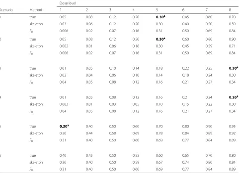
Table 1Six toxicity scenarios for a single-agent trial withθ=0.3
Dose level
Scenario Method 1 2 3 4 5 6 7 8
1 true 0.05 0.08 0.12 0.20 0.30a 0.45 0.60 0.70
skeleton 0.03 0.06 0.12 0.20 0.30 0.40 0.50 0.59
F0 0.006 0.02 0.07 0.16 0.31 0.50 0.69 0.84
2 true 0.05 0.08 0.12 0.20 0.30a 0.60 0.80 0.90
skeleton 0.002 0.01 0.06 0.16 0.30 0.45 0.59 0.71
F0 0.006 0.02 0.07 0.16 0.31 0.50 0.69 0.84
3 true 0.01 0.05 0.10 0.14 0.18 0.22 0.25 0.30a
skeleton 0.02 0.04 0.06 0.10 0.14 0.18 0.24 0.30
F0 0.04 0.05 0.08 0.12 0.16 0.21 0.27 0.34
4 true 0.01 0.05 0.08 0.12 0.16 0.2 0.24 0.26a
skeleton 0.003 0.01 0.03 0.05 0.10 0.15 0.22 0.30
F0 0.04 0.05 0.08 0.12 0.16 0.21 0.27 0.34
5 true 0.30a 0.40 0.50 0.60 0.70 0.80 0.90 0.95
skeleton 0.30 0.44 0.58 0.69 0.78 0.84 0.89 0.92
F0 0.31 0.40 0.50 0.60 0.69 0.77 0.84 0.89
6 true 0.40 0.45 0.50 0.55 0.60 0.65 0.70 0.80
skeleton 0.30 0.40 0.50 0.59 0.67 0.74 0.80 0.84
F0 0.31 0.40 0.50 0.60 0.69 0.77 0.84 0.89
aNumbers in boldface are the target MTDs
probability never reaching unacceptable levels, and there is no target dose but level 8 is quite close to the target dose given in Scenario 3; Scenario 5 implies that all the dose levels have an unacceptable toxicity probability, and the target dose is level 1; Scenario 6 is used to examine the situation that all the doses are over toxic, and there is no target dose but level 1 is quite close to the target dose. In practice, the trial would be stopped and doses will be reformulated once too many toxicities are occurred. We take sample size of each trial asN = 60, the number of cohorts asJ=20, andm=3. In implementing the Gibbs sampler, we collect 1000 observations after 700 burn-in iterations.
For comparison, we consider two Bayesian model-based CRM dose-finding methods including the power model: pi = dexpi (β) and one-parameter logistic model: pi = exp(a0+βdi)/{1+exp(a0+βdi)}with a0 = 3, where
the prior ofβis assumed to follow the normal distribution with mean zero and variance 1.34, i.e.,β∼N(0, 1.34). For each of the above considered six scenarios, givenθ,kand
K, a good “skeleton” can be directly generated using the function ‘getprior’ in the R package with the optimal value ofδ, which can be obtained by the algorithm of Lee and Cheung [17]. But, its computational burden is too expen-sive. To address this issue, we here use a fixed value, which is evaluated using the data-dependent approach via sim-ulation studies from a prespecified indifference interval so that the trial has some desirable operating character-istics, for example, the prior expectation ofηis close to its true values, to replace the optimal value ofδ. For our considered six scenarios, simulation studies evidence that we can take δ as 0.05, 0.075, 0.03, 0.04, 0.07 and 0.05, respectively.
For each of the above considered six scenarios, we set the initial value p(0)as its corresponding skeleton in implementing Gibbs sampler. WhenαandF0are assumed
Table 2Bayesian estimates ofpk’s via NCRM under scenario 1
True 0.05 0.08 0.12 0.20 0.30 0.45 0.60 0.70
i xi yi1 yi2 yi3 pˆ1 pˆ2 pˆ3 pˆ4 pˆ5 pˆ6 pˆ7 pˆ8
1 d1 0 0 1
2 d1 0 0 0 0.0156 - - -
-3 d2 0 0 0 0.0278 0.0380 - - -
-4 d3 1 0 0 0.0439 0.0573 0.0789 - - - -
-5 d4 0 0 0 0.0501 0.0703 0.1014 0.1336 - - -
-6 d5 0 0 0 0.0585 0.0809 0.1169 0.1534 0.2109 - -
-7 d6 0 0 1 0.0589 0.0852 0.1248 0.1682 0.2377 0.3426 -
-8 d5 0 1 0 0.0595 0.0734 0.1196 0.1672 0.2430 0.3457 -
-9 d6 1 1 1 0.0711 0.1018 0.1496 0.2006 0.2841 0.4060 -
-10 d5 0 1 0 0.0763 0.0954 0.1484 0.2023 0.2864 0.4063 -
-11 d5 0 1 1 0.0681 0.0995 0.1528 0.2112 0.3116 0.4156 -
-12 d5 0 0 1 0.0814 0.1144 0.1668 0.2227 0.3190 0.4196 -
-13 d4 0 0 0 0.0702 0.0979 0.1474 0.1965 0.3072 0.4144 -
-14 d5 0 0 1 0.0670 0.0979 0.1431 0.1958 0.3104 0.4151 -
-15 d5 0 0 0 0.0672 0.0960 0.1421 0.1915 0.2904 0.4062 -
-16 d5 0 0 1 0.0767 0.1073 0.1549 0.2026 0.2989 0.4094 -
-17 d5 0 1 0 0.0704 0.1004 0.1450 0.1941 0.2958 0.4070 -
-18 d5 1 1 0 0.0723 0.1039 0.1546 0.2066 0.3196 0.4205 -
-19 d4 0 0 0 0.0632 0.0916 0.1369 0.1842 0.3128 0.4170 -
-20 d5 0 0 0 0.0730 0.1046 0.1428 0.1868 0.2977 0.4103 -
-1 1.5 2 2.5 3 3.5 4 4.5 5 5.5 6 0
0.1 0.2 0.3 0.4 0.5
1 2 3 4 5 6 7 8 0
0.05 0.1 0.15 0.2 0.25 0.3 0.35
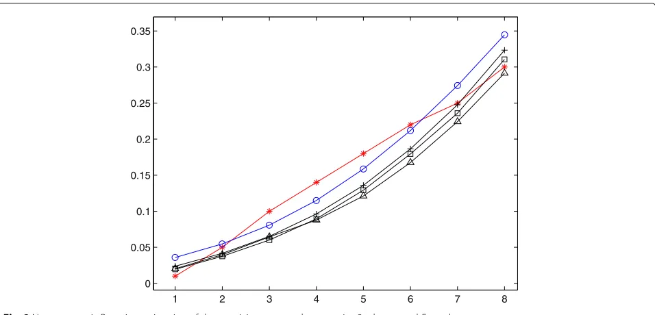
Fig. 2Nonparametric Bayesian estimation of dose-toxicity curve under scenarios 3 whenαandF0are known
F0. As mentioned above, we choose appropriate values
of μ and σ such that median of F0 should be
consis-tent with the initial guess for the MTD. To wit, if there is a prior belief that dose level dk is the MTD, we can select appropriate values of μandσ such thatF0(dk|η)=
dk−μ
σ
=θ. Table1gives the values ofF0’s
correspond-ing to six scenarios together with eight dose levels, where μ=6 andσ =2 for scenario 1 and 2,μ=10 andσ =5 for scenario 3 and 4, andμ=3 andσ =4 for scenario 5 and 6, respectively.
The preceding proposed hybrid algorithm is used to cal-culate Bayesian estimates ofpk’s, and the preceding pro-posed two-stage Bayesian nonparametric adaptive dose-finding algorithm is employed to determine MTD. To illustrate how the NCRM works, we present results of one simulation trial for scenario 1 together with α = 5 in Table 2. Included in this table are: i (the serial number of the current experiment cohort); xi (the dose admin-istered to the current cohort of patients); yi1, yi2, yi3
(the observations for the current experiment cohort);pˆk (estimate of toxicity probability fork = 1,. . .,K). Exam-ination of Table 2 shows that (i) dose level 5 (i.e., d5)
is selected as the MTD and pˆ5 = 0.2977, which is
quite close to true toxicity probability 0.3; (ii) among 11 cohorts of patients administered to dose level d5,
only 10 patients (i.e., 20i=13m=1yim) are experienced toxicity; (iii) the doses with the relatively high toxicity probability (such as d7 andd8) may have no chance to
be administered to patients, which guarantees the safety of patients.
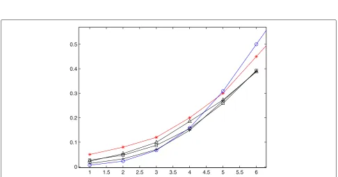
Figures 1 and 2 plot Bayesian nonparametric estima-tions of unknown dose-toxicity curve for three speci-fied values of α for scenarios 1 and 3, respectively. In each figure, “−” represents the dose-toxicity curve cor-responding to true dose-toxicity data, “−◦” corresponds to the base curve, and “− ”, “−” and “-+” corre-spond to the estimated dose-toxicity curves for α = 5, 10 and 20, respectively. Examination of Figs. 1 and 2 show that the estimated curves are more and more close to F0 with the increase of α when the doses
adminis-tered to patients are less than but close to the target dose, which is consistent with the conclusion that the large value of α reflects a prior belief that F is tight aroundF0.
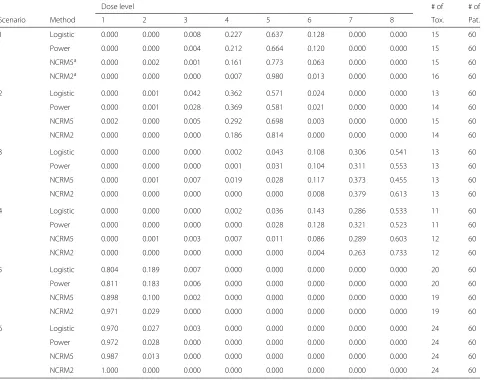
Table 3Selection probabilities and total numbers of toxicities observed for logistic model, power model and NCRM under six scenarios
Dose level # of # of
Scenario Method 1 2 3 4 5 6 7 8 Tox. Pat.
1 Logistic 0.000 0.000 0.008 0.227 0.637 0.128 0.000 0.000 15 60
Power 0.000 0.000 0.004 0.212 0.664 0.120 0.000 0.000 15 60
NCRM5a 0.000 0.002 0.001 0.161 0.773 0.063 0.000 0.000 15 60
NCRM2a 0.000 0.000 0.000 0.007 0.980 0.013 0.000 0.000 16 60
2 Logistic 0.000 0.001 0.042 0.362 0.571 0.024 0.000 0.000 13 60
Power 0.000 0.001 0.028 0.369 0.581 0.021 0.000 0.000 14 60
NCRM5 0.002 0.000 0.005 0.292 0.698 0.003 0.000 0.000 15 60
NCRM2 0.000 0.000 0.000 0.186 0.814 0.000 0.000 0.000 14 60
3 Logistic 0.000 0.000 0.000 0.002 0.043 0.108 0.306 0.541 13 60
Power 0.000 0.000 0.000 0.001 0.031 0.104 0.311 0.553 13 60
NCRM5 0.000 0.001 0.007 0.019 0.028 0.117 0.373 0.455 13 60
NCRM2 0.000 0.000 0.000 0.000 0.000 0.008 0.379 0.613 13 60
4 Logistic 0.000 0.000 0.000 0.002 0.036 0.143 0.286 0.533 11 60
Power 0.000 0.000 0.000 0.000 0.028 0.128 0.321 0.523 11 60
NCRM5 0.000 0.001 0.003 0.007 0.011 0.086 0.289 0.603 12 60
NCRM2 0.000 0.000 0.000 0.000 0.000 0.004 0.263 0.733 12 60
5 Logistic 0.804 0.189 0.007 0.000 0.000 0.000 0.000 0.000 20 60
Power 0.811 0.183 0.006 0.000 0.000 0.000 0.000 0.000 20 60
NCRM5 0.898 0.100 0.002 0.000 0.000 0.000 0.000 0.000 19 60
NCRM2 0.971 0.029 0.000 0.000 0.000 0.000 0.000 0.000 19 60
6 Logistic 0.970 0.027 0.003 0.000 0.000 0.000 0.000 0.000 24 60
Power 0.972 0.028 0.000 0.000 0.000 0.000 0.000 0.000 24 60
NCRM5 0.987 0.013 0.000 0.000 0.000 0.000 0.000 0.000 24 60
NCRM2 1.000 0.000 0.000 0.000 0.000 0.000 0.000 0.000 24 60
aNCRM5 and NCRM2 denote NCRM method withα=5 and 20, respectively
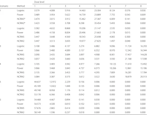
the total number of toxicities observed are almost iden-tical for all three methods under our considered cases; (iv) Bayesian NCRM has a higher percentage of patients treated at MTD than two parametric CRMs, except for scenario 3 with α = 5, but Bayesian NCRM treats more patients at dose levels below MTD and less patients at dose levels above MTD than two parametric CRMs; (v) the selection probabilities for scenarios 3 and 4 are smaller than those for other four scenarios because the locations of target doses for scenarios 3 and 4 are dif-ferent from those for other scenarios, which indicates that the highest dose should be carefully administered to patients for safety, and patients should be administered to the lower dose level.
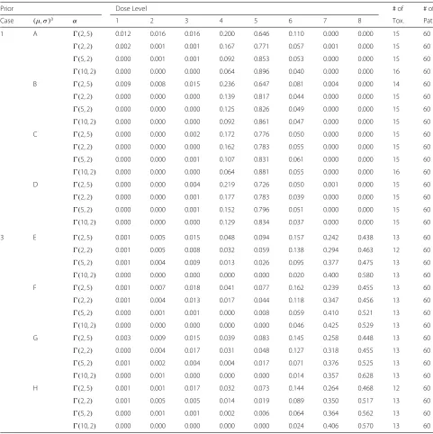
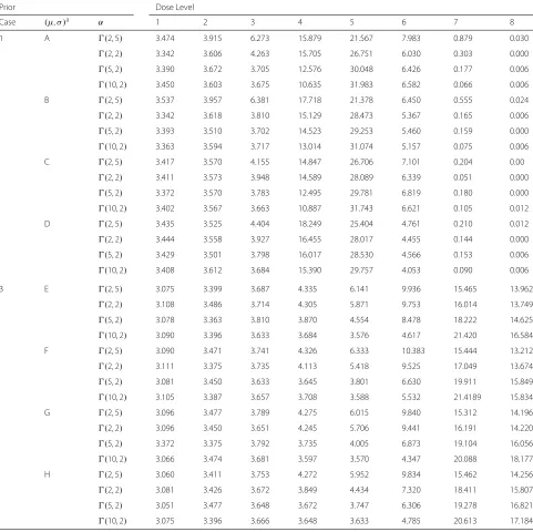
Now we assume that α and F0 are unknown. As an
illustration of the above presented Bayesian NCRM proce-dure, here we only consider scenarios 1 and 3. For scenario 1, we consider four different priors onα:(2, 5),(2, 2),
(5, 2)and(10, 2), which correspond to small and mod-erate expectations ofα, and four discrete uniform priors for(μ,σ )on the rectangles(5, 7)×(1, 3),(4, 8)×(1, 3), (5, 7)×(0, 4)and(4, 8)×(0, 4), which indicate that prior expectations ofμandσ are 6 and 2, respectively. For sce-nario 3, we consider the same priors onα as scenario 1, but the following four different discrete uniform priors of (μ,σ ) on the rectangles (9, 11)× (4, 6), (8, 12) ×(4, 6), (9, 11)×(3, 7)and(8, 12)×(3, 7), which imply that prior expectations ofμandσare 10 and 5, respectively.
Table 4Average numbers of patients treated at each of eights doses for logistic model, power model and NCRM
Dose level
Scenario Method 1 2 3 4 5 6 7 8
1 Logistic 3.579 4.008 5.916 14.463 23.304 8.124 0.576 0.030
Power 3.489 3.954 5.622 14.739 23.889 7.755 0.543 0.009
NCRM5a 3.474 3.615 3.912 15.462 27.387 6.009 0.141 0.000
NCRM2a 3.423 3.558 3.708 8.298 35.454 5.493 0.066 0.000
2 Logistic 3.582 4.632 8.868 19.206 21.147 2.535 0.030 0.000
Power 3.486 4.158 8.004 20.496 21.663 2.178 0.015 0.000
NCRM5 3.447 3.648 4.569 18.543 25.698 4.065 0.300 0.000
NCRM2 3.447 3.513 3.693 19.977 27.825 1.497 0.048 0.000
3 Logistic 3.108 3.486 4.137 5.274 6.882 9.096 11.724 16.293
Power 3.066 3.480 4.089 5.157 6.552 8.970 12.342 16.344
NCRM5 3.090 3.435 3.684 3.897 4.908 8.901 17.457 14.628
NCRM2 3.057 3.420 3.660 3.636 3.531 3.930 21.168 17.598
4 Logistic 3.105 3.483 3.942 4.977 7.266 10.125 11.610 15.492
Power 3.066 3.468 3.843 4.737 6.573 10.266 12.861 15.186
NCRM5 3.135 3.366 3.453 3.777 4.395 7.809 16.281 17.784
NCRM2 3.084 3.387 3.573 3.612 3.522 3.630 18.879 20.313
5 Logistic 44.637 12.972 2.229 0.156 0.006 0.000 0.000 0.000
Power 45.189 12.822 1.848 0.135 0.006 0.000 0.000 0.000
NCRM5 49.740 8.958 1.176 0.114 0.012 0.000 0.000 0.000
NCRM2 53.178 6.366 0.408 0.042 0.006 0.000 0.000 0.000
6 Logistic 54.468 4.467 0.894 0.141 0.030 0.000 0.000 0.000
Power 54.573 4.500 0.810 0.102 0.015 0.000 0.000 0.000
NCRM5 57.676 2.865 0.414 0.039 0.006 0.000 0.000 0.000
NCRM2 58.149 1.596 0.237 0.018 0.000 0.000 0.000 0.000
aNCRM5 and NCRM2 denote NCRM method withα=5 and 20, respectively
3. Results for 1000 simulated trials are given in Tables5 and 6. Examination of Table 5 and6 shows that (i) the selection probabilities and the number of patients treated at the MTD increase with the increase of prior expecta-tion ofα; (ii) the selection probabilities and the number of patients treated at the dose level closet to the MTD decrease with the increase of prior expectation ofα for scenario 1, but increase with the increase of prior expecta-tion ofαfor scenario 3; (iii) the total number of toxicities observed are almost equal regardless of the priors ofαand (μ,σ ), which shows that there is little effect of the selec-tion of the priors ofα,μ andσ on the total number of toxicities observed.
Results
According to the above presented simulation study, we have the following results. First, the estimated MTD in single-agent dose-finding clinical trials via our proposed two-stage Bayesian nonparametric adaptive dose-finding
Table 5Selection probabilities and total numbers of toxicities observed for NCRM under scenarios 1 and 3 whenαand(μ,σ )are unknown
Prior Dose Level # of # of
Case (μ,σ )a α 1 2 3 4 5 6 7 8 Tox. Pat.
1 A (2, 5) 0.012 0.016 0.016 0.200 0.646 0.110 0.000 0.000 15 60
(2, 2) 0.002 0.001 0.001 0.167 0.771 0.057 0.001 0.000 15 60
(5, 2) 0.000 0.001 0.001 0.092 0.853 0.053 0.000 0.000 15 60
(10, 2) 0.000 0.000 0.000 0.064 0.896 0.040 0.000 0.000 16 60
B (2, 5) 0.009 0.008 0.015 0.236 0.647 0.081 0.004 0.000 14 60
(2, 2) 0.000 0.000 0.000 0.139 0.817 0.044 0.000 0.000 15 60
(5, 2) 0.000 0.000 0.000 0.125 0.826 0.049 0.000 0.000 15 60
(10, 2) 0.000 0.000 0.000 0.092 0.861 0.047 0.000 0.000 15 60
C (2, 5) 0.000 0.000 0.002 0.172 0.776 0.050 0.000 0.000 15 60
(2, 2) 0.000 0.000 0.000 0.162 0.783 0.055 0.000 0.000 15 60
(5, 2) 0.000 0.000 0.001 0.107 0.831 0.061 0.000 0.000 15 60
(10, 2) 0.000 0.000 0.000 0.064 0.881 0.055 0.000 0.000 16 60
D (2, 5) 0.000 0.000 0.004 0.219 0.726 0.050 0.001 0.000 15 60
(2, 2) 0.000 0.000 0.001 0.177 0.783 0.039 0.000 0.000 15 60
(5, 2) 0.000 0.000 0.001 0.152 0.796 0.051 0.000 0.000 15 60
(10, 2) 0.000 0.000 0.000 0.129 0.834 0.037 0.000 0.000 15 60
3 E (2, 5) 0.001 0.005 0.015 0.048 0.094 0.157 0.242 0.438 13 60
(2, 2) 0.001 0.005 0.008 0.032 0.059 0.138 0.294 0.463 12 60
(5, 2) 0.001 0.004 0.009 0.013 0.026 0.095 0.377 0.475 13 60
(10, 2) 0.000 0.000 0.000 0.000 0.000 0.020 0.400 0.580 13 60
F (2, 5) 0.001 0.007 0.018 0.041 0.077 0.162 0.239 0.455 13 60
(2, 2) 0.001 0.004 0.013 0.017 0.044 0.118 0.347 0.456 13 60
(5, 2) 0.000 0.001 0.001 0.000 0.008 0.059 0.410 0.521 13 60
(10, 2) 0.000 0.000 0.000 0.000 0.000 0.046 0.425 0.529 13 60
G (2, 5) 0.003 0.009 0.015 0.039 0.083 0.145 0.258 0.448 13 60
(2, 2) 0.000 0.004 0.017 0.031 0.048 0.127 0.318 0.455 13 60
(5, 2) 0.001 0.002 0.004 0.004 0.017 0.071 0.376 0.525 13 60
(10, 2) 0.000 0.001 0.000 0.000 0.000 0.014 0.357 0.628 13 60
H (2, 5) 0.001 0.001 0.017 0.032 0.073 0.144 0.264 0.468 12 60
(2, 2) 0.001 0.005 0.005 0.014 0.019 0.089 0.350 0.517 13 60
(5, 2) 0.000 0.001 0.001 0.002 0.006 0.064 0.364 0.562 13 60
(10, 2) 0.000 0.000 0.000 0.000 0.000 0.024 0.406 0.570 13 60
aNote:A=(5, 7)×(1, 3),B=(4, 8)×(1, 3),C=(5, 7)×(0, 4),D=(4, 8)×(0, 4),E=(9, 11)×(4, 6),F=(8, 12)×(4, 6),G=(9, 11)×(3, 7),H=(8, 12)×(3, 7)
Discussion
Although this manuscript only considers a single agent dose-finding design, the proposed Bayesian NCRM can be extended to two-agent dose-finding studies, which is our further research topic. On the other hand, this paper only considers the evaluation of the toxicity of novel drug treatment, i.e., phase I clinical trial, but the developed Bayesian NCRM procedure can be extended to Bayesian nonparametric phase I/II dose-finding trial design that
simultaneously allows for toxicity and efficiency of novel drug treatment for precision medicine.
Conclusions
Table 6Average numbers of patients treated at each of eight doses for NCRM under scenario 1 and 3 whenαand(μ,σ )are unknown
Prior Dose Level
Case (μ,σ )a α 1 2 3 4 5 6 7 8
1 A (2, 5) 3.474 3.915 6.273 15.879 21.567 7.983 0.879 0.030
(2, 2) 3.342 3.606 4.263 15.705 26.751 6.030 0.303 0.000
(5, 2) 3.390 3.672 3.705 12.576 30.048 6.426 0.177 0.006
(10, 2) 3.450 3.603 3.675 10.635 31.983 6.582 0.066 0.006
B (2, 5) 3.537 3.957 6.381 17.718 21.378 6.450 0.555 0.024
(2, 2) 3.342 3.618 3.810 15.129 28.473 5.367 0.165 0.006
(5, 2) 3.393 3.510 3.702 14.523 29.253 5.460 0.159 0.000
(10, 2) 3.363 3.594 3.717 13.014 31.074 5.157 0.075 0.006
C (2, 5) 3.417 3.570 4.155 14.847 26.706 7.101 0.204 0.00
(2, 2) 3.411 3.573 3.948 14.589 28.089 6.339 0.051 0.000
(5, 2) 3.372 3.570 3.783 12.495 29.781 6.819 0.180 0.000
(10, 2) 3.402 3.567 3.663 10.887 31.743 6.621 0.105 0.012
D (2, 5) 3.435 3.525 4.404 18.249 25.404 4.761 0.210 0.012
(2, 2) 3.444 3.558 3.927 16.455 28.017 4.455 0.144 0.000
(5, 2) 3.429 3.501 3.798 16.017 28.530 4.566 0.153 0.006
(10, 2) 3.408 3.612 3.684 15.390 29.757 4.053 0.090 0.006
3 E (2, 5) 3.075 3.399 3.687 4.335 6.141 9.936 15.465 13.962
(2, 2) 3.108 3.486 3.714 4.305 5.871 9.753 16.014 13.749
(5, 2) 3.078 3.363 3.810 3.870 4.554 8.478 18.222 14.625
(10, 2) 3.090 3.396 3.633 3.684 3.576 4.617 21.420 16.584
F (2, 5) 3.090 3.471 3.741 4.326 6.333 10.383 15.444 13.212
(2, 2) 3.111 3.375 3.735 4.113 5.418 9.525 17.049 13.674
(5, 2) 3.081 3.450 3.633 3.645 3.801 6.630 19.911 15.849
(10, 2) 3.105 3.387 3.657 3.708 3.588 5.532 21.4189 15.834
G (2, 5) 3.096 3.477 3.789 4.275 6.015 9.840 15.312 14.196
(2, 2) 3.096 3.450 3.651 4.245 5.706 9.441 16.191 14.220
(5, 2) 3.372 3.375 3.792 3.735 4.005 6.873 19.104 16.056
(10, 2) 3.066 3.474 3.681 3.597 3.570 4.347 20.088 18.177
H (2, 5) 3.060 3.411 3.753 4.272 5.952 9.834 15.462 14.256
(2, 2) 3.081 3.426 3.672 3.849 4.434 7.320 18.411 15.807
(5, 2) 3.051 3.477 3.648 3.672 3.747 6.306 19.278 16.821
(10, 2) 3.075 3.396 3.666 3.648 3.633 4.785 20.613 17.184
aNote:A=(5, 7)×(1, 3),B=(4, 8)×(1, 3),C=(5, 7)×(0, 4),D=(4, 8)×(0, 4),E=(9, 11)×(4, 6),F=(8, 12)×(4, 6),G=(9, 11)×(3, 7),H=(8, 12)×(3, 7)
distribution of dose-toxicity curve. A Bayesian method is developed to estimate toxicity probabilities of dose levels considered. A hybrid algorithm combining the Gibbs sampler and adaptive rejection Metropolis sam-pling algorithm is developed to generate observations from joint conditional distributions required in evaluating Bayesian estimates of toxicity probabilities of dose levels. A two-stage Bayesian nonparametric adaptive dose-finding design is developed to estimate the MTD. In the
Abbreviations
ARMS: Adaptive rejection Metropolis sampling; CRM: Continual reassessment method; DP: Dirichlet process; DLT: Dose-limiting toxicity; MTD: Maximum tolerated dose; NCRM: Nonparametric Continual reassessment method
Acknowledgements
The authors are grateful to the Editor, an Associate Editor and two referees for their valuable suggestions and comments for largely improving the manuscript.
Funding
This work was supported by the grants from the National Natural Science Foundation of China (Grant No.: 11671349) and the Key Projects of the National Natural Science Foundation of China (Grant No.: 11731101).
Availability of data and materials
The datasets generated and analysed during the current study are available from the corresponding author on reasonable request.
Authors’ contributions
NST conceived of research questions, developed methods and revised the manuscript; SJW carried out statistical analysis and drafted the manuscript; GY conducted simulation studies. All authors commented on successive drafts, and read and approved the final manuscript.
Ethics approval and consent to participate
Not applicable.
Consent for publication
Not applicable.
Competing interests
The authors declare that they have no competing interests.
Publisher’s Note
Springer Nature remains neutral with regard to jurisdictional claims in published maps and institutional affiliations.
Received: 29 May 2018 Accepted: 1 November 2018
References
1. O’Quigley J, Pepe M, Fisher L. Continual reassessment method: a practical design for phase 1 clinical trials in cancer. Biometrics. 1990;46:33–48. 2. Whitehead J, Brunier H. Bayesian decision procedures for dose
determining experiments. Stat Med. 1995;14:885–93.
3. Piantadosi S, Fisher JD, Grossman S. Practical implementation of a modified continual reassessment method for dose-finding trials. Cancer Chemother Pharmacol. 1998;41:429–36.
4. Heyd JM, Carlin BP. Adaptive design improvements in the continual reassessment method for phase I studies. Stat Med. 1999;18:1307–21. 5. Leung DH, Wang YG. An extension of the continual reassessment
method using decision theory. Stat Med. 2002;21:51–63.
6. Yuan Z, Chappell R, Bailey H. The Continual Reassessment Method for Multiple Toxicity Grades: A Bayesian Quasi ikelihood Approach. Biometrics. 2007;63:173–9.
7. Yin G, Yuan Y. Bayesian Model Averaging Continual Reassessment Method in Phase I Clinical Trials. J Am Stat Assoc. 2009;104:954–68. 8. Møller S. An extension of the continual reassessment methods using a
preliminary up-and-down design in a dose finding study in cancer patients, in order to investigate a greater range of doses. Stat Med. 2010;14:911–22.
9. Fan SK, Lu Y, Wang YG. A simple Bayesian decision-theoretic design for dose-finding trials. Stat Med. 2012;31:3719–30.
10. Morita S, Thall PF, Takeda K. A simulation study of methods for selecting subgroup-specific dosesin phase i trials. Pharm Stat. 2017;16:143–56. 11. Gelfand AE, Kuo L. Nonparametric bayesian bioassay including ordered
polytomous response. Biometrika. 1991;78:657–66.
12. Mukhopadhyay S. Bayesian nonparametric inference on the dose level with specified response rate. Biometrics. 2000;56:220–6.
13. Gasparini M, Eisele J. A curve-free method for phase i clinical trials. Biometrics. 2000;56:609–15.
14. Cheng YK. Dose Finding by the Continual Reassessment Method. Boca Raton: Chapman and Hall/CRC; 2011, pp. 57–62.
15. Ivanova A, Wang K. Bivariate isotonic design for dose-finding with ordered groups. Stat Med. 2006;25:2018–26.
16. Yan F, Mandrekar SJ, Yuan Y. Keyboard: a novel bayesian toxicity probability interval design for phase i clinical trials. Clin Cancer Res Off J Am Assoc Cancer Res. 2017;23:3994–4003.
17. Lee SM, Cheung YK. Modal calibration in the continual reassessment method. Clin Trials. 2009;6:227–38.
18. Ramsey FL. A Bayesian approach to bioassay. Biometrics. 1972;28:841–58. 19. Escobar MD, West M. Bayesian density estimation and inference using
mixtures. Publ Am Stat Assoc. 1995;90:577–88.