http://www.sciencepublishinggroup.com/j/jfa doi: 10.11648/j.jfa.20170501.15
ISSN: 2330-7331 (Print); ISSN: 2330-7323 (Online)
Econometric Analysis of Local Government Investment
Efficiency and the Debt Risk Based on the DSGE Model
Zhi-qi Zhu
1, Ke Gao
2, Tao Wang
2, Nan Bai
31Tianjin University of Finance and Economics, Tianjin, P. R. China 2
Central University of Finance and Economics, Beijing, P. R. China 3Renmin University of China, Beijing, P. R. China
Email address:
zhuzhiqi12345@163.com (Zhi-qi Zhu), gkfly@126.com (Ke Gao), manutdwangtao@126.com (Tao Wang), 99536157@qq.com (Nan Bai)
To cite this article:
Zhi-qi Zhu, Ke Gao, Tao Wang, Nan Bai. Econometric Analysis of Local Government Investment Efficiency and the Debt Risk Based on the DSGE Model. Journal of Finance and Accounting. Vol. 5, No. 1, 2017, pp. 56-60. doi: 10.11648/j.jfa.20170501.15
Received: November 30, 2016; Accepted: February 3, 2017; Published: March 1, 2017
Abstract:
This paper examines the relationship between the efficiency of government investment and the debt risk from a theoretical perspective. By building a DSGE model, we introduced the impact of government financial investment, and investigated the change of debt risk under different government investment efficiency. From the model, we observed a obvious reverse effect bwteen the the government investment efficiency and debt risk. Finally, according to research conclusions, we put forward some Suggestions.Keywords:
DSGE Model, Local Government Debt, Government Investment Efficiency, Government Debt Risk1. Introduction
In response to the impact of the economic crisis in 2008, the Chinese government launched an emergency 4 trillion investment plan and with the loose monetary policy. The central government had supported local government to increase investment and financing platform to issue bonds. This investment-driven way would smooth economic fluctuations. These measures maked our country's economy was the first to stabilize and rise. Also, these measures maked up the short board of the infrastructure construction in our country. However, with the stabilization of China's economy, the policy had also caused two more serious problems. First, the local government could not directly borrow. By establishing financing platforms and other means of curve financing, local government obtained higher cost of funds, while leaving a large number of debt outside the budget supervision. Second, there was a partial pursuit of local government GDP growth phenomenon. There were a large number of low returns, low positive externalities of investment. It is also worth noting that there are some interaction mechanisms between these two problems.
In 2015, the Ministry of Finance estimated that Chinese government’s debt ratio rosed to 41.5%, lower than the
standard 60% (the Treaty of Maastricht). With the fiscal policy becoming the mainstay of steady growth, the budget deficit rate increased from 2.2% to 3% in 2016. Therefore, it is necessary to clarify the relationship between government investment efficiency and debt risk. In this paper, we hope to establish the DSGE model to analyze the mechanism of government expenditure efficiency and the debt risk.
2. DSGE Model and Analysis
This paper constructs a closed DSGE model, which includes households, firms, central bank, and the financial sector. Assuming that families are free to choose consumption, labor supply and government bond holdings to achieve intertemporal maximization. Manufacturers are intermediate goods manufacturers and final product manufacturers, their goals are to pursue cost minimization and profit maximization. Intermediate goods manufacturers are in a monopolistic competitive market, and the final products are in a completely competitive market. The interest rate rule is formulated by the central bank, and the financial rules are formulated by the government.
A. Households
Here h is the consumption habit, is the weight parameter of labor supply, is composed of public goods and private goods consisting a group of consumer bundle, The equation is as follows:
Here is the proportion of private goods consumption, v is the substitution elasticity between public goods consumption and private goods consumption. Budget constraint conditions:
Household income comes from after-tax wages, after-tax capital gains, after-tax bond income, transfer payments and corporate dividends. Households spend mainly on consumption, investing and buying government bonds. Where is the capital utilization, is the depreciation, is the tax rate. The form of the capital accumulation equation is as follows:
According to Christiano (2005) settings, we assume that the form of investment adjustment costs are as follows:
According to Leeper (2010), we set the depreciation form as follows:
By maximizing the utility function, the First Order Condition (FOC) of the variable can be obtained:
Here 、 are Lagrangian multipliers, is
Tobin's q value, is t period inflation index. B. Sticky Salary Setting
Drawing on Erceg et al. (2000), we assume that each household is a monopoly provider of different labor. is providing labor. And [0, 1]. The aggregate form of heterogeneous labor is as follows:
Here is the alternative elasticity of the different labor force. The demand function of the individual labor force is obtained by maximizing profit:
Bring zero profit to condition, and obtained:
We introduce the Calvo (1983) method to achieve the sticky wage setting. Suppose that each period has a fixed probability that the family can change the wage. In order to maximize the expected utility, the family develops the optimal form of sticky wage as follows:
Solve the real optimal sticky wage:
According to the formula (14), we write the real wage as an exponential form:
C. Final Product Manufacturers
We set the production function of the final goods manufacturer as Dixit-Stiglitz function.
D. Intermediate Goods Manufacturers
We set the intermediate goods manufacturer's production function as C-D function.
Here is the public capital stock, is the output elasticity of public capital. . is total factor productivity. We set it to the AR (1) procedure:
Intermediate goods manufacturers pursue cost minimization.
Solve the real wage and real capital returns are as follows:
Referring to the Calvo (1983) hypothesis, we will set the probability of intermediate goods companies changing-price as . The probability that firm k does not adjust prices is
. The sticky price setting takes the form:
Solve the optimal price of viscous intermediate and write the form of inflation:
The price index equation is written in the form of inflation:
E. Central Bank
We assume that the central bank follows the Taylor rule and focuses on interest rate adjustment.
Here Rs is the steady-state interest rate, is the steady-state inflation, and is the steady-state output. Parameter determines the smoothness of the interest rate. and determine the extent to which interest rates
deviate from the steady state for inflation and output. F. Financial Department
We set the budget in the form of a balance as follows:
Government revenue comes from taxes and bonds, spending for government consumption, government investment, transfer payments and repayment of the previous debt. The form of government public capital accumulation is as follows:
Here, is the depreciation rate of public capital, we assume that the government's investment adjustment cost form the same as private capital.
For the sake of generality, we refer to Schwarzmuller's (2015) fiscal rule set.
Here, represents the debt ratio of the government in
period t. is the adjustment
parameter of the fiscal policy to the economic growth, and is the adjustment parameter of the fiscal policy to the debt ratio deviating from the steady state. is the financial impact, subject to AR (1) process.
G. Parameter Calibration
calibration value of is 0.75. The alternative elasticity of the intermediate product is 10 (Zhang Zuomin, 2014). The elasticity of labor is 3. The reciprocal of labor supply elasticity is 2.16. And the calibration value of the alternative elasticity of private goods and public goods consumption is 0.8. According to Wang Wenfu's (2010) study, the monetary policy adjustment parameter calibration value =0.92, =1.766, =0.2533. The proportion of private goods consumption in the total consumption of is 0.8. Referring to Wang and Yang's (2014) study, we set the steady-state tax rate calibration value =0.0937, =0.1007, =0.2851. By calculating the average of government consumption and
government investment as a proportion of GDP from 2010 to 2014, the calibration value of is 0.135 and the calibration value of is 0.116. There is no consensus on the margin of safety of debt, so we use the "Maastricht Treaty" standard, the debt ratio of the steady-state value is calibrated to 60%. To ensure that each financial repayment rule has a steady state solution, we adjust the fiscal policy smoothing parameter to 0.35 and the fiscal policy
adjustment parameter to 0.45.
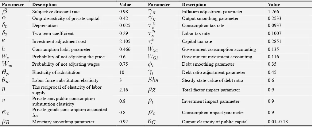
The assignment of the relevant parameters is shown in Table 1.
Table 1. Parameter Calibration Table.
Parameter Description Value Parameter Description Value
Subjective discount rate 0.98 Inflation adjustment parameter 1.766 Output elasticity of private capital 0.42 Output smoothing parameter 0.2533 Depreciation 0.025 Consumption tax rate 0.0937
Two term coefficient 0.29 Labor tax rate 0.1007
Investment adjustment cost 2.105 Capital tax rate 0.2851
Consumption habit parameter 0.466 Government consumption accounting 0.135 Probability of not adjusting the price 0.6 Government investment accounting 0.116 Probability of not adjusting wages 0.75 Debt smoothing parameter 0.35
Elasticity of substitution 10 Debt ratio adjustment parameter 0.45
Labor force substitution elasticity 3 Steady-state value of debt ratio 0.6 The reciprocal of elasticity of labor
supply 2.16 Total factor impact parameter 0.9 Private and public consumption
substitution elasticity 0.8 Investment impact parameter 0.9 Private goods consumption accounted
for 0.8 Consumption impact parameter 0.9 Monetary smoothing parameter 0.92 Output elasticity of public capital 0.01~0.18
H. Numerical Simulation
In order to use this model to examine the relationship between government investment efficiency and debt risk, we must choose the relevant indicators in the model as proxy variables of government investment efficiency and debt risk. Because the efficiency of government investment lies in its promoting effect on output, we use the output elasticity of public capital to represent the efficiency of government investment. At present, the main way to measure the debt risk is to investigate the fluctuation of the debt. So we use the standard deviation of the debt ratio under the impact of government investment to represent the debt risk. He Gang, Chen Wenjing (2008); Yang Feihu, Zhou Quanlin (2013) estimated that China's public capital output elasticity of 0.18
or less. Therefore, we examine the fluctuation of the corresponding elasticity of public capital output from 0.01 to 0.18.
We introduce fiscal investment shocks to represent the relationship between government investment efficiency and debt risk. Figure 1 shows the relationship between the elasticity of public capital output and the standard deviation of debt ratios. It can be seen from the figure that with the increase of public capital output elasticity, the fluctuation of debt ratio under the impact of financial investment is getting smaller and smaller. The government investment efficiency and the debt risk have the reverse change relations, the government investment efficiency is higher, the debt risk is lower.
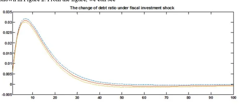
In order to reflect the fluctuation difference of debt ratio under different government investment efficiency level, we take the elasticity of public capital output as 0.05, 0.1 and 0.5 respectively. The impact of different debt ratio fluctuations in the situation is shown in Figure 2. From the figure, we can see
that under different conditions of the output elasticity of public capital, the fluctuation of the liability rate caused by the impact is different. The higher the elasticity of public capital output, the smaller the fluctuation of debt ratio.
Figure 2. Debt Rate of Impact.
3. Conclusion and Suggestion
This paper examines the relationship between the efficiency of government investment and the debt risk from a theoretical perspective. By constructing a DSGE model, we can observe that there is a significant negative correlation between the efficiency of government investment and the risk of debt. Chinese economy is currently facing downward pressure. Government debt burdens are on the rise. The task of resolving the government debt risk is urgent.
This paper proposes to resolve the local government debt risk by controlling the efficiency of government investment. Improve the efficiency of government investment from government debt investment "stock" and "incremental" two aspects.
On the one hand, we need to improve the efficiency of local government’s "stock" investment. At present, the problem of excess capacity in China is still grim. We need to remove the excess capacity, promote the optimization and adjustment of economic structure. We need to strengthen government budget management. We need to strictly follow the requirements of the new budget law, strengthen supervision and management, strengthen budget constraints.
On the other hand, we need to improve the efficiency of government’s "incremental" investment. We must clarify the government and market boundaries. We must optimize the government investment structure. We need to focus our investments primarily on where the market fails. We need to protect the public sector investment, while continuing to vigorously promote the PPP project.
References
[1] Calvo G A. Staggered prices in a utility-maximizing framework [J]. Journal of monetary Economics. 1983, 12 (3): 383-398.
[2] Christiano L J, Eichenbaum M, Evans C L. Nominal rigidities and the dynamic effects of a shock to monetary policy [J]. Journal of political Economy. 2005, 113 (1): 1-45.
[3] Erceg C J, Henderson D W, Levin A T. Optimal monetary policy with staggered wage and price contracts [J]. Journal of monetary Economics. 2000, 46 (2): 281-313.
[4] Greiner A, Wendroff J H. Electrospinning: A Fascinating Method for the Preparation of Ultrathin Fibers [J]. Cheminform. 2007, 38 (42): 5670-5703.
[5] Leeper E M, Plante M, Traum N. Dynamics of fiscal financing in the United States [J]. Journal of Econometrics. 2010, 156 (2): 304-321.
[6] Prescott E C. Why do Americans work so much more than Europeans? [R]. National Bureau of Economic Research, 2004. [7] Reinhart C M, Rogoff K S. Growth in a time of debt (digest summary) [J]. American Economic Review. 2010, 100 (2): 573-578.
[8] Schwarzmüller T, Wolters M H. The short-and long-run effects of fiscal consolidation in dynamic general equilibrium [C]. 2014.
[9] Zhong-xia Jin. Real Interest Rates, Real Wages and Economic Restructuring—Analysis Based on DSGE [J]. China Economist, 2014,(02):46-56.