Vol.8 (2018) No. 5
ISSN: 2088-5334
Real Time Monocular Visual Odometry Using Hybrid Features
and Distance Ratio for Scale Estimation
Diky Septa Nugroho
#, Igi Ardiyanto
#*, Adha Imam Cahyadi
# #Department of Electrical Engineering and Information Technology, Faculty of Engineering, Universitas Gadjah Mada, Yogyakarta, Indonesia
E-mail: [email protected]
Abstract— Real-time dead reckoning navigation is important for supplying information on the current position of an autonomous
mobile robot to complete its task, especially in certain areas such as hazardous and GPS-denied areas. Monocular visual odometry is a good choice as it is one of the dead reckoning navigation methods, which only uses a single camera. For real-time task, visual odometry requires fast feature extraction without ignoring its accuracy. Therefore, we propose the usage of a hybrid feature, i.e., Censure feature detector and upright SURF feature descriptor, as feature extraction. The scale ambiguity for the monocular visual odometry becomes a challenging problem. Without 85 Part 1 - 27 Paper additional information from other sensors, estimating the scale is solely the only way. In our proposed work, distance ratio is employed to tackle such problems. Experimental results show the performance of the designed algorithm. A real example of running the proposed algorithm under an embedded device is also provided for demonstrating its real-time capability.
Keywords— visual odometry; distance ratio; scaling factor; Censure; upright SURF.
I. INTRODUCTION
Nowadays, the development of a mobile robot is very fast due to its various deployment in a vast kind of applications, ranging from surveillance to the high-risk missions. Information of the current position is one of an important thing for the mobile robot. In certain areas such as hazardous and GPS-denied areas, mobile robots are required to be aware of their current position. Dead reckoning navigation is one of the most commonly used technique with massive kind of sensors to solve the problem. Among these sensors, the camera becomes an exciting option because it provides rich information, yet it is very cheap.
Estimating the ego-motion, i.e., the position and orientate ion, using frame series of one camera or more is called visual odometry (VO) [1]. In general, the visual odometer algorithm consists of three steps; extracting the features, matching, and estimating the camera pose. Later, the feature extraction incorporates feature detection and description. Camera pose estimation can be done using feature correspondence between two consecutive frames by solving the epipolar constraint.
Different schemes of VO have been developed. These different schemes include Kinect based VO [2], monocular VO, and multicamera VO. However, most of works on VO used monocular vision [3]-[6]) and stereo vision [7] -[9].
In this work, we try to alleviate the limitations from the previous mentioned approaches above. Our main contribution lies in the usage of hybrid feature detectors and its combination with distance ratio for solving the camera scale problems. Here we employ Censure feature detector and Upright SURF as feature descriptor. These algorithms are employed due to their fast computation and stability to detect the same feature across viewpoint change [14] [15]. Furthermore, the scale ambiguity for the monocular visual odometry, which becomes a challenging problem in a normal case is diminished using distance ratio method.
II. MATERIAL AND METHOD
A. Modeling the Camera
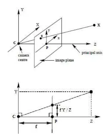
Here we assume a pinhole camera model, as shown in Fig. 1.
Fig. 1 Geometry of pinhole camera, where C describes the camera center and p denotes the principal point.
X represents the world point denoted by the homogeneous
4-vector (X, Y, Z, 1)T, x is image point denoted by a homogeneous 3-vector, and P is the homogeneous camera projection matrix. Subsequently, the projected image point is
= P (1)
Projection matrix P consists of internal and external camera parameters. The internal camera parameters consist of focal length f, and principle point (pxpx, ) in a matrix K. While the external camera parameters consist of camera orientation R and camera position t in world coordinate system.
(2)
Subsequently, equation (1) can be expressed as
(3)
B. Censure Feature Detector
Fig. 2 Center surround filter for the proximation of Laplacian used in Censure
The main reason for choosing this feature detector is it has good stability, accuracy, and computation time. All of them are the recipe to make a good real-time task like visual odometry [14].
There are several steps to detect features from the image, first is to calculate the extrema in a local neighborhood using a simplified center-surround filter in all scales. Finally, the extremes are filtered by taking out the weak corner responses of the Harris measurement.
Approximation of laplacian employs bi-level multiplication by either 1 or −1. Figure 2 shows the center-surround filters used here that is a circle with two overlapping squares: upright and 45 degrees rotated, where every scale is denoted by different block size n.
Bi-level filter is the key for Censure because of its efficiency. The box filter is calculated by integral images [16]. Since the filter shape is a polygon, we employ an extended version of integral images. Each trapezoidal area is calculated using two different slanted of the integral images, where the summation of pixels denotes an angled area. Parameter α is used to control the degree of slant (skew)
(4)
Where α = 0 represents the standard rectangular integral image. When α < 0, the summed area skews to the left, and reciprocally. (Fig. 3 left).
Fig. 3 Skewed integral images for building trapezoidal áreas.
Afterward, a response is subdued when optimal responses appear in a local neighborhood since it will be repeatable. Alternatively, unstable. Features on an edge or line are also not stable. Thus, a threshold is applied to remove those responses. The second-moment matrix of the response function is employed to remove these responses.
(5)
obtained, its trace and determinant are employed to calculate the ratio of principal curvatures.
C. Upright Surf Descriptor
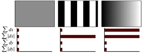
Computing SURF descriptor requires two steps: obtaining a consistent orientation using information from a circular region of the interesting point and constructing a square region aligned up to the chosen orientation. Here we utilize the upright version of SURF descriptor (U-SURF) which is variant to the image rotation and faster to calculate.
Extracting the descriptors requires building a square region centered on the interesting point, with a window size of 20x20. The region is separated into smaller 4×4 square regions for keeping important information. In each sub-region, we calculate several simple features at 5×5 and its Haar wavelet responses in horizontal direction dx and vertical direction day. The robustness to geometric deformations and localization errors is increased by giving weight to dx and dy response with a Gaussian (σ = 3.3s) (see Fig. 4).
Afterward, the summation of the wavelet responses dx and dy in each sub region becomes the feature vector. For considering the polarity information of the change in intensity, the summation of |dx| and |dy| is extracted. Subsequently, each sub region has a four-dimensional descriptor vector v for its intensity structure v = (dx, dy, |dx|, |dy|)T. It yields a descriptor vector of length 64 for each interest point.
Fig. 4 The descriptor denotes the nature of the underlying intensity pattern. Left: all values are low for the homogeneous region. Middle: when there are frequencies in x-direction, the value of |dx| is high. Right: when the intensity is increasing in x-direction, dx and |dx| are high.
D. Camera Pose Estimation
Monocular visual odometry uses the series of images denoted by 0, …, where k is the kth image taken by camethe ra. For simplifying the problem, we assume the camera coordinate frame similar to the agent’s coordinate frame. Transformation of two consecutive camera positions at time k - 1 and k is denoted by , −1 ∈ ℝ4×4 of the following form
(6)
Where , −1 ∈ (3) denotes the rotation matrix, and , −1
∈ ℝ3×1 is the translation vector. Then, the camera poses 0, … , contains the relative camera pose transformation to the initial coordinate frame at 0. In this work, 0 is at the origin of the camera coordinate frame.
The computation of transformation Tk between two images
and −1 can be done by using two sets of corresponding
features −1, from each image. In this work, both −1, and are described in 2-D coordinates.
Two consecutive images and −1 of a calibrated camera are geometrically related and the relationship is defined by the essential matrix E. Essential matrix conceives the camera rotation and translation parameters with unknown scale translation factor in the following form
(7)
where and
(8)
Since the scale factor is unknown, the symbol ≅ is used. The essential matrix is calculated using only 2-D feature correspondences of two consecutive images. After all element of E are in the rotation and translation matrix can be obtained. Therefore, computation of essential matrix is the most important step. As we stated before, geometry relation in the form of essential matrix E is obtained from geometry constraint called epipolar constraint, specifying the line on which the corresponding feature point of resides in the other image. This constraint can be defined by
(9)
where denotes a feature location in an image (e.g., Ik) and represents the location of its corresponding feature in
another image, Ik-1). and are in the form .
By using eight-point algorithm [17], each matched feature gives a constraint of the following form
(10)
where = [ 1 2 3 4 5 6 7 8 9]T
If there are eight points pair and each pair give a constraint, by stacking the constraints we obtain a linear equation system AE = 0, and the parameters of E can be calculated by solving the system.
E. Algorithm Design
In this work, we design a scale estimation algorithm for monocular visual odometry as shown in Fig. 5. The first step is initialization, which is initialized by inputting the first image from KITTI dataset. Since the distortion effect of the image generated from the KITTI data has already been removed, no preprocessing of the image is required. Subsequently, the next step is the feature detection using Censure. As mentioned in the previous section, there are several parameters, which must be set. The filter response threshold is set to 20, to produce the stable feature, local neighborhood extrema selection at 3x3x3 to produce more feature, and we use 30 as the size of n blocks. After that, the feature detected is described by using the upright-SURF descriptor.
up a feature in the first descriptor set. Subsequently, it is fitted with all other features in the second set. Ratio test is applied to remove the bad match. [18]. Later, we calculate the essential matrix based on feature correspondences.
Fig. 5 Algorithm flowchart
As mentioned above, the main problem here is that the monocular scheme is up to scale. Therefore, the distance of the translation movement has to be known by using external information like IMU, or GPS. However, in this work, the only sensor used is the camera. However, it is possible to calculate relative scales for the subsequent transformations. A possible solution is by triangulating 3-D points Xk-1 and Xk from two subsequent images, and computing combination of two 3-D points to obtain the relative distances. The scale is then calculated from the distance ratio r between a pair (Xk, Yk) and a point pair (Xk-1, Yk-1) (see Fig. 6). Since the computation produces a relative scale, the first scale of the movement has to be known. Therefore, ground truth at C1 and C2 is used to get this information. These approaches are borrowed from Scaramuzza et al. [1].
Fig. 6 Illustration of distance ratio
(11)
However, there is a difference between the same 3D point that reconstructed from a different image pair. The far object like the sky or the dynamic objects like car or person can cause this difference. Thus, we have to remove this outlier. In this work, a simple Random Sampling Consensus [19] method is employed. A set of feature correspondence is triangulated so there are I correspondence 3-D points. Subsequently, the distance between two correspondence 3-D points di is computed. Two of them will be chosen randomly. Linear line model is used by joining the chosen point. Then the data that lies inside a certain threshold from the line is called support. This step is repeated until n iteration. A pair of data that produce the most support is chosen to remove the outlier (see Fig. 7).
Fig. 7 RANSAC illustration. The black dot is supported, and the red one is an outlier.
After we get the relative scale, the final camera poses in term of rotation and translation matrix in k frame Rk, and task can be obtained by concatenating the previous transformation
and .
(12)
(13)
III.RESULTS AND DISCUSSION
The performance of the proposed visual odometry algorithm with scale estimation is measured by comparing with that algorithm without scale estimation and the ground truth. First, images from sequence00 KITTI dataset are used to test the algorithm. These datasets contain a set of images taken by a rigidly attached camera on a car in an urban area. The images are saved in 8-bit PNG. For diminishing the Get next Image Ik
Feature detection and description
Feature matching Ik and Ik-1
Compute essential matrix E for image pair
Ik and Ik-1
Decompose rotation R and translation t from E
Estimate relative scale and rescale t
Second image?
Concacenate Rk,k-1 and
tk,k-1 to get Rk and tk
Get absolute distance and rescale t first
image?
No Yes
Yes
distortion effect, the images are cropped with the size smaller than the original 1392 x 512 pixels. KITTI dataset also provides both external and internal camera calibration matrix. Test results include rotational and translational comparisons.
As shown in Fig. 8a, the trajectory that constructed by our algorithm is closer to the ground truth than the visual odometry without scale estimation. However the translational error generated by our algorithm is still quite high. This can be caused by the scale estimation when there is a slight translational movement with considerable rotation, which is not too big. So, the algorithm at that time yields a big drift. However, in translational movement, our algorithm gives a good performance. Scale estimation using distance ratio from 3D points obtained through the process of triangulation is still the weakness of this method. It is inevitable that the fact is the closer the two frames to triangulation, the greater the uncertainty of the resulting 3D point.
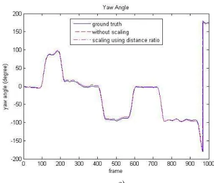
As shown in Fig. 8c we can see that the translational movement only affects the scale. The orientation of the camera is still the same because the sequences are a planar motion on xz plane, and the only considered Euler angle is the yaw angle. In this case, our algorithm gives auspicious results.
a)
b)
c)
Fig. 8 Simulation result on a) camera trajectory. b) translational error. c) yaw angle trajectory
TABLEI AVERAGE COMPUTATION TIME
Number of iteration Computation time (ms)
10 308.14
20 318.38
30 329.08
40 344.18
50 359.8
60 369.24
70 390.06
80 403.18
90 407.86
100 438.28
110 513.08
Accuracy and computation time are the most important for a real-time navigation algorithm like visual odometry. Both of them cannot be optimized simultaneously. Therefore, there must be compensation between them. RANSAC for outlier removal is an iterative method, so we must test the relationship between the number of iteration and the accuracy represented by the translational error. Here, we limit the computation time up to 500 ms due to the real-time purpose. The iteration test is set from 0 to 100 with ten additional iterations on each test.
The test is done by comparing the translational error from two different iterations. We use a hypothesis that the bigger the number of iteration the smaller the translational error generated. We subsequently write the hypothesis in the following form
(14) (15)
(16)
Where and
are the mean
of absolute translational errors, and are standard deviations, and is some frames. Index 1 represents the fewer iteration, and 2 represent the bigger iteration. We can conclude that we accept our hypothesis HA if z computed is bigger than zα where α is significance level which means the probability of the wrong conclusion.TABLEII
HYPOTHESIS TESTS THE DIFFERENCE BETWEEN TWO TRANSLATIONAL ERROR MEANS FROM TWO DIFFERENT ITERATION
Iteration 10 20 30 40 50 60 70 80 90 100
10 0 0 1 1 1 0 0 1 1
20 0 1 1 1 1 1 1 1
30 1 1 1 1 1 1 1
40 0 0 0 0 1 0
50 0 0 0 1 0
60 0 0 1 1
70 1 1 1
80 1 1
90 0
100
From Table II, to conclude that the hypothesis is correct, all of the hypothesis tests should accept the formulated hypothesis. This study found that there is no sufficient evidence to say that the hypothesis is true. The results show that few of points is sufficient to compute the distance ratio. However, we can find that the best iteration, which outperformed the others, is those who have a most accepted hypothesis in the vertical and most rejected hypothesis in horizontal, i.e., 40 and 90. This iteration can be used in further applications.
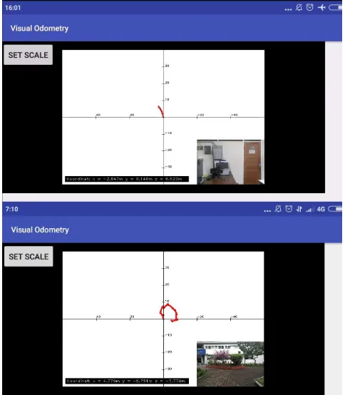
Afterward, the designed algorithm is implemented on an embedded system, i.e. Smartphone to check the performance of the algorithm. The first test is a straight movement with 6 meters along the z-axis and the second test is movement around the hexagonal park. Because the ground truth is unknown, we use to start and end position in the same place. The test results as shown in Fig. 9 show that the absolute error of the last camera pose generated by the application in the first test is 2.9 m, and the second test is 7.832 m. Average computation time taken by the first test is 1564.08, and 2609.28 ms for the second test. Computation time taken by the application is slower than computation time taken in the simulation test because CPU speed of Smartphone is lower than PC. This result shows that the application is still far away to be ready to use. So further development to reduce the computation and reduce the absolute error of the camera pose is needed.
Fig. 9 Visual odometry application interface for the first test (top) and the second test (bottom).
IV.CONCLUSIONS
The scale estimated by our algorithm can reduce the error significantly, although the error still appears. For future work, another sensor like IMU or GPS to solve the problem can fuse visual odometry. However, our algorithm has good accuracy in the rotation since the Censure feature is proven rotation invariant. Also, computation time taken by the whole algorithm is still high because of brute force feature matching. Therefore, the other feature matching methods should be investigated to make the computation time faster.
ACKNOWLEDGMENT
We would like to thank Causal Productions for permits to use and revise the template provided by Causal Productions. Original version of this template was provided by courtesy of Causal Productions (www.causalproductions.com).
REFERENCES
[1] D. Scaramuzza and F. Fraundorfer, ”Visual Odometry: Part I: The First 30 Years and Fundamentals,” IEEE Robotics & Automation Magazine, vol 18, no. 4, Dec.2011, pp. 80-92.
[2] H. Yu, H. Sun, Y. Wang, L. Kan and Q. Wan, "An improved visual odometry optimization algorithm based on Kinect camera," 2013 Chinese Automation Congress, Changsha, 2013, pp. 691-696. [3] T. Kanade, “Transforming camera geometry to a virtual downward
looking camera: robust ego-motion estimation and ground-layer detection,” in 2003 IEEE Computer Society Conference on Computer Vision and Pattern Recognition, 2003. Proceedings. IEEE Comput. Soc, 2003, pp. I–390–I–397.
[4] S. Lovegrove, A. J. Davison, and J. Ibanez-Guzman, “Accurate visual odometry from a rear parking camera,” in 2011 IEEE Intelligent Vehicles Symposium (IV). IEEE, Jun. 2011, pp. 788–793. [5] Y. Yu, C. Pradalier, and G. Zong, “Appearance-based monocular
[6] A. Cumani, “Feature Localization Refinement for Improved Visual Odometry Accuracy,” Int. Jour. Circuits, Systems and Signal Processing, vol. 5, no. 2, pp. 151–158, 2011.
[7] D. Nist´er, O. Naroditsky, and J. Bergen, “Visual odometry,” in Proceedings of the 2004 IEEE Computer Society Conference on Computer Vision and Pattern Recognition, 2004. CVPR 2004., vol. 1. Ieee, 2004, pp. 652–659.
[8] B. Kitt, A. Geiger, and H. Lategahn, “Visual odometry based on stereo image sequences with RANSAC-based outlier rejection scheme,” in 2010 IEEE Intelligent Vehicles Symposium. IEEE, Jun. 2010, pp. 486–492.
[9] A. Geiger, J. Ziegler, and C. Stiller, “Stereoscan: Dense 3d reconstruction in real-time,” in Intelligent Vehicles Symposium (IV), 2011 IEEE, pp. 963–968.
[10] S. Choi, J. Park, and W. Yu, "Resolving scale ambiguity for monocular visual odometry," 2013 10th International Conference on Ubiquitous Robots and Ambient Intelligence (URAI), Jeju, 2013, pp. 604-608.
[11] F. Fraundorfer, D. Scaramuzza, and M. Pollefeys, "A constricted bundle adjustment parameterization for relative scale estimation in visual odometry," 2010 IEEE International Conference on Robotics and Automation, Anchorage, AK, 2010, pp. 1899-1904.
[12] A. T. N. Nishitani and D. F. Wolf, "Solving the Monocular Visual Odometry Scale Problem with the Efficient Second-Order Minimization Method," 2015 12th Latin American Robotics Symposium and 2015 3rd Brazilian Symposium on Robotics (LARS-SBR), Uberlandia, 2015, pp. 126-131.
[13] D. Zhou, Y. Dai, and H. Li, "Reliable scale estimation and correction for monocular Visual Odometry," 2016 IEEE Intelligent Vehicles Symposium (IV), Gothenburg, 2016, pp. 490-495.
[14] M. Agrawal, K. Konolige, and M. Blas, “Censure: Center surround extremes for realtime feature detection and matching,” in Proc. European Conf. Computer Vision, 2008, pp. 102–115.
[15] H. Bay, A. Ess, T. Tuytelaars, and L. Van Gool, “SURF: Speeded up robust features,” Computer Vision and Image Understanding (CVIU), vol. 110, no. 3, pp. 346–359, 2008.
[16] P. Viola and M. Jones, “Robust real-time face detection,” In: ICCV 2001.
[17] H. Longuet-Higgins, “A computer algorithm for reconstructing a scene from two projections,” Nature, vol. 293, no. 10, pp. 133–135, 1981.
[18] D. G. Lowe. Distinctive image features from scale-invariant keypoints. International Journal of Computer Vision, 60(2):91-110, 2004.