Single-Loop Optimization for Losses Minimization in Medium-Voltage Power Distribution System

Vol.7 (2017) No. 4

ISSN: 2088-5334

Single-Loop Optimization for Losses Minimization in

Medium-Voltage Power Distribution System

Teguh Utomo

, Rini Nur Hasanah

, Muhammad Fahmy Madjid

Electrical Engineering Department, Brawijaya University, Jalan MT Haryono 167, Malang, 65145, Indonesia E-mail: [email protected]; [email protected]

Abstract— One important goal during the reconfiguration of a medium-voltage power distribution network is to minimize the

active-power losses of the system. Therefore, the objective function of an optimization problem would represent the total active-power losses of the distribution system, by considering only the active component of power losses while ignoring the reactive part. Constraints would be load flow, voltage drop, and the network configuration. In this paper, losses problem during the reconfiguration of a medium-voltage power distribution system have been minimized using a single-loop optimization method, whereas the load-flow analysis has been performed by utilizing the Newton-Raphson method. The optimization method was aimed to minimize the active-power losses of the system by formulating the problem as a matter of network reconfiguration. The solution scheme has been begun with a mesh distribution-network which had been obtained previously by assuming all the switches to be closed and then opened sequentially to eliminate loops. The optimization results showed that in a 21-bus distribution system there had been 10800 combinations, in which the lowest power losses occurred under the combination of NO 23, NO 21, NO 22, NO 24, NO 25, whereas the combination of NO 7, NO 10, NO 20, NO 15, NO 20, resulted in the power losses of 0.1676 per unit, being equal to 16.76 kVA at the base power of 100 kVA.

Keywords— Losses minimization; power distribution system; single loop optimization.

I. INTRODUCTION

The primary distribution network is a part of the electric power transmission system, extending from the medium-voltage substation to the primary winding-part of the distribution transformer. It can be represented by the diagram in Fig. 1.

Fig. 1 Diagram of a primary distribution network [1]

As seen in Fig. 1, the first layer a represents the substations or switchyards, being linked using the primary distribution line b to the busbars c, and furthermore the distribution transformers d, secondary distribution network e, and the load/customers f. Such system is defined as a

radial system, although it can be in a closed-loop or mesh network.

In a power delivery system, the distribution system occupies the most important place. Its service quality can be guaranteed if several requirements, such as continuity of service (related to disturbance conditions) and flexibility to load growth (under normal operating conditions), are met. However, it is not a simple matter to fulfill all those requirements in a distribution system, considering the variability of the technical and economic aspects of all load conditions. This is due to differences in load density and load placement situations, which in turn leads to high losses of power from the network and overloads on the network.

Some researchers have attempted to minimize the power losses of the system by formulating the problem as a matter of reconfiguring the distribution network [2]-[14]. Initial works on the network reconfiguration to reduce the losses was presented in [4]-[8]. The proposed solution was started from the distribution system mesh, which had been previously obtained by assuming all switches to be closed and opened sequentially to eliminate the loop.

on the development of the method in [5], the research in [6] created a heuristic method by introducing two approaches to the power-flow during the system load transfer.

Other research papers specifically proposed the optimization and heuristic methods for the reconfiguration of distribution networks by including current constraints and feeder voltages [10]-[12]. The compensation principle was based on the power-flow technique to ensure that the strength of the weak distribution-network mesh could be modeled more accurately. A two-level algorithm concept which was based on the modified and simulated annealing techniques and the use of epsilon-constraint method (ε) to solve the distribution network reconfiguration problem was introduced in [13]-[14].

II. MATERIAL AND METHOD

A. Power-Flow Analysis

The method proposed in this article was based on the use of power-flow analysis using the Newton-Raphson method [15]-[29] and holomorphic embedding method [26]-[29]. The power-flow study is aimed at calculating the voltage, current, and power at various locations of a power system under steady-state operation, whether in existing condition or to be expected to occur in the future. In a power system, the power flows from the generating plants to the customer’s locations through a transmission system. In this process, many things need attention including the voltage of each bus, the active and reactive power flow (in MW and MVAR) of each line, and others.

Each bus in a power network system includes the values of active power (P), reactive power (Q), the magnitude of the voltage (E), and the phase angle (θ). These variables are required to evaluate the performance of the power system and to analyze the generation and loading conditions. In the power-flow equation, two of those variables are known, whereas the others are to be determined.

The buses in a power system can be classified into three types of bus [17]-[20]:

• Load Bus (PQ bus)

• Generator Bus (PV bus)

• Swing/slack Bus

The known components in a load bus are the active power P and the reactive power Q, while the quantities to determine are the voltage E and the phase angle θ. In a generator bus, the known components are the magnitude of voltage E and the active power P, whereas the quantities to determine are the phase angle θ and the reactive power Q. In a slack bus, the known components are the magnitude of the

voltage E and the phase angle θ, whereas the unknowns are

the active power P and the reactive power Q.

Generally, in the power-flow study, there is only one swing bus. The swing bus serves to supply the lack of active power P and the reactive power Q in the system. The power system comprises several buses interconnected with each other. The electric power which is injected by the generator into certain bus can be absorbed not only by the load connected to the bus but also by the load on another bus. The excess of power on one bus will be transferred through the transmission line to other power-deficient buses.

B. The Prevailing Equations in Power-Flow Analysis

By referring to Fig. 2, the relationship among parameters and variables in a power system can be expressed in the form of admittance as expressed in Eq. (1) [17],[18].

bus bus

bus Y E

I = (1)

where

Ibus : current matrix on each bus

Ybus : admittance matrix

Ebus : voltages matrix on each bus

Fig. 2 Model of a transmission line for power-flow calculation ([17]-[20])

Computation iteration must be carried out to find out the value of the voltage on each bus. Iteration is to be done until the results difference between two consecutive iterations is less than or equal to some predetermined error value. The obtained result will be the voltage values on each node. The power on each bus is also to be computed iteratively. Eq. (2) represents the power calculation on each bus [17]-[21].

* x _p

p p

p jQ E I

P + = (2)

where

Pp : active power on the p-bus

Qp : reactive power on the p-bus

Ep : voltage on the p-bus

Ipq : current from the p-bus

Besides determining the power on each bus, load-flow analysis also serves to find the losses during the power transmission from the generating stations to the load centres. As being referred in Fig. 2, the line current Ipq is found on

the p-bus and the associated positive direction of current is from p to q, as expressed in Eq. (3).

(

)

p L

pq I I y E -E y E

I = + 0= + 0 (3)

where

IL : current on the line between the pth-bus and the qth

-bus

Ip0 : current on the line of half-line charging

ypq : line admittance between the pth-bus and the qth-bus

yp0 : half-line charging

Eq : voltage on the q th

-bus

Oppositely, the line current Iqp is measured on the qth-bus

and the associated positive direction of current is from q to p, as expressed in Eq. (4).

(

)

q L

qp I I y E -E y E

I =− + ₀= + ₀ (4)

The complex power Spq from the p th

-bus to the qth-bus, and Sqp from the qth-bus to the pth-bus, are expressed in Eqs.

(5) and (6).

* x _pq

p

pq E I

S = (5)

* x _qp

q

qp E I

The power losses in the line p-q are obtained from the algebraic sum of power in Eqs. (5) and (6), as stated in Eq. (7).

qp pp

Lpq S S

S = + (7)

so that the total power losses of the considered line containing n buses can be represented by Eq. (8).

∑∑

SLpq : power losses of the line between the pth-bus and

the qth-bus SLT : total power losses

C. The Utilization of Newton-Raphson Method

The problem of load-flow analysis can be solved using the Newton-Raphson method [15]-[21]. It is performed by exploring a number of nonlinear equations which represent the active and reactive powers as functions of the voltage magnitude and phase angle. The power on the ith-bus can be formulated as:

∑

i jQ E I E Y E

P

1 *

* ₍₉₎

By separating the real part from the imaginary part, the following equations are obtained.

        =

∑

i E Y E

P 1 * Re (10)         − =

∑

i E Y E

Q

1 *

Im (11)

Both the nonlinear equations for the Pi and Qi become the

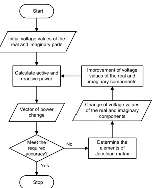
principal equations in the load-flow analysis using the Newton-Raphson method. Two nonlinear equations are resulted on each bus. The active and reactive powers are known, whereas the magnitude and the phase-angle of the voltage are to be found on all buses except the slack bus. The voltage of the slack bus is known and kept constant so that there are 2(n-1) equations to be solved in the load-flow calculation. The flowchart to find the bus voltage using the Newton-Raphson method is given in Fig. 3.

Start

Initial voltage values of the real and imaginary parts

Calculate active and reactive power

Vector of power change Meet the required accuracy? Determine the elements of Jacobian matrix Change of voltage values

of the real and imaginary components Improvement of voltage

values of the real and imaginary components

Stop Yes

No

Fig. 3 A flow-chart to find the bus voltage using the Newton-Raphson method

D. Single-Loop Optimization Method

Using the known data, the simulation of power flow

calculation is done using Newton-Raphson and

Holomorphic Embedding method. Power flow analysis simulation is done using following steps:

1) Determining the number of buses to be simulated 2) Collecting the data of active and reactive powers on

each bus

3) Modeling the system based on the related single-line diagram

4) Assigning the value of each component according to the data source

5) Determining the error value to be considered for iteration in load-flow analysis

6) Performing the load-flow analysis using the Newton-Raphson method

7) Performing the load-flow analysis using the Holomorphic Embedding method

8) Performing the analysis on the results, computation time and complexity for single-loop optimization method.

The load-flow analysis results are furthermore used to explore and elaborate the main focus of the research problem, including the computation time as well as the implementation complexity of the single-loop optimization method by using the objective function and the network constraints as follows:

2 f fI

R [P]

Min =

∑

Subject to:

Radial configuration constraint

1

ft =

Π_{λ (13)}

Drop voltage constraint

max ij, ij V V ≤∆

∆ (14)

Load flow constrain

max ij, ij S

S ≤ (15)

where

P : power losses of the network system

∆Vij : voltage drop on the line i-j

Sij : load flow on the line i-j

ft

λ

Π _{: radiality of the primary distribution network}

system (λft is 0 if switch is closed, 1 if switch is open)

The algorithm to solve the problem of distribution network reconfiguration for power losses minimization using the single-loop optimization method can be explained as follows:

1) Solving the radial distribution network problem. 2) Creating a loop by switching on the NO switches if

power losses minimization is desired.

3) Determining the optimum flow of the loop obtained in Step 2.

4) Computing the load-flow using topology technique or Newton-Raphson methods

5) Restoring the radial configuration of the distribution network

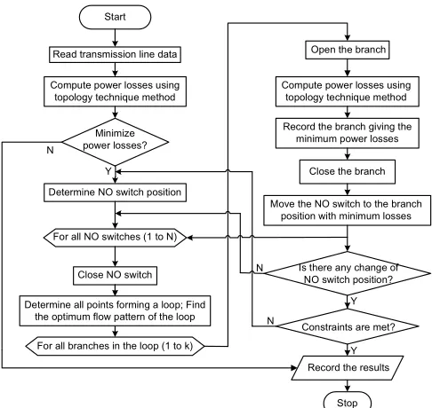
The detail steps of power losses minimization using the single-loop optimization method based on the topology technique calculation are given in the flowchart of Fig. 4.

Start

Read transmission line data

Compute power losses using topology technique method

Minimize power losses?

Determine NO switch position

Close NO switch For all NO switches (1 to N)

Determine all points forming a loop; Find the optimum flow pattern of the loop

For all branches in the loop (1 to k)

Open the branch

Compute power losses using topology technique method

Record the branch giving the minimum power losses

Close the branch

Move the NO switch to the branch position with minimum losses

Is there any change of NO switch position?

Constraints are met?

Record the results

Stop Y

N

Y N

Y N

Fig. 4 A flow-chart of the single-loop optimization method for distribution network reconfiguration

III.RESULTS AND DISCUSSION

As a case study of the implementation of the proposed method, a system with 21 buses has been taken. Fig. 5 indicates the initial configuration of the 21-bus electrical distribution system, whereas Fig. 6 represents its containing loops.

Fig. 5 The initial configuration of the 21-bus electrical distribution system

Fig. 6 The initial configuration of the 21-bus electrical distribution system with loops

The single-line diagram contains Normally-Open (NO) and Normally-Close (NC) switches, with buses are indicated with numbers, as shown in Fig. 7.

Fig. 7 The initial configuration of the 21-bus electrical distribution system being completed with branch numbers

A. The Considered 21-bus Network System

As shown in Fig. 5, the system contains 21 buses, consisting of one generator-bus, 20 load-buses, and 25 distribution lines. The generator of the distribution system comprises one swing bus. Bus #1 is the swing bus, and the other buses are the bus load (PQ bus).

The parameters of lines between buses in the 21-bus system are given in Table 1. The data consist of resistance (R), reactance (X), and the half-line charging (1/2 yc), all

being in per units.

TABLE I

DATA OF THE LINES BETWEEN BUSES

Sending bus

Receiving

bus R (p.u.) X (p.u.) 1/2yc 1 2 0.0000153 0.0000145 0.0000000 2 3 0.0000969 0.0000922 0.0000000 2 4 0.0005733 0.0005454 0.0000000 2 8 0.0000728 0.0000692 0.0000000 2 12 0.0000585 0.0001423 0.0000000 4 5 0.0000958 0.0000912 0.0000000 5 6 0.0000915 0.0000870 0.0000000 6 7 0.0001084 0.0001031 0.0000000 8 9 0.0001155 0.0001098 0.0000000 9 10 0.0001318 0.0001254 0.0000000 10 11 0.0000706 0.0000672 0.0000000 12 13 0.0001670 0.0001589 0.0000000 12 14 0.0001896 0.0001803 0.0000000 14 15 0.0001496 0.0001423 0.0000000 15 16 0.0001806 0.0001718 0.0000000 15 17 0.0002105 0.0002001 0.0000000 15 19 0.0001197 0.0001138 0.0000000 17 18 0.0001906 0.0001813 0.0000000 19 20 0.0001347 0.0007885 0.0000000 20 21 0.0002713 0.0002577 0.0000000 3 10 0.0002000 0.0002000 0.0000000 5 21 0.0002000 0.0002000 0.0000000 7 11 0.0002000 0.0002000 0.0000000 13 16 0.0002000 0.0002000 0.0000000 18 21 0.0002000 0.0002000 0.0000000

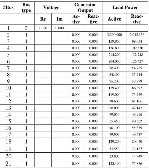
The voltage value is given in per unit (p.u.), whereas the power is stated in kVA. The per unit value of power has been obtained using the base power (kVA base), which was 100 kVA.

TABLE II

DATA OF GENERATOR AND LOAD OF EACH BUS

#Bus Bus

type Voltage

Generator

Output Load Power

Re Im

Ac-tive

Reac-tive Active

Reac-tive

1 3 1.000 0.000

2 1 0.000 0.000 3.300.000 2.045.156 3 1 0.000 0.000 159.800 99.034 4 1 0.000 0.000 176.800 109.570 5 1 0.000 0.000 214.200 132.748 6 1 0.000 0.000 204.000 126.427 7 1 0.000 0.000 88.400 54.785 8 1 0.000 0.000 54.400 33.714 9 1 0.000 0.000 95.200 58.999 10 1 0.000 0.000 139.400 86.392 11 1 0.000 0.000 119.000 73.749 12 1 0.000 0.000 98.600 61.106 13 1 0.000 0.000 68.000 42.142 14 1 0.000 0.000 79.050 48.996 15 1 0.000 0.000 65.450 40.562 16 1 0.000 0.000 90.100 55.839 17 1 0.000 0.000 79.900 49.517

18 1 0.000 0.000 129.200 80.070

19 1 0.000 0.000 53.550 33.187

20 1 0.000 0.000 23.800 14.749

21 1 0.000 0.000 122.400 75.856

B. Results of Simulation

Using the 21-bus system, the optimization calculation has been carried out in 10800 iterations or 10800 combinations of NO-NC switch, whose results sample capture is given in Table 3. The load-flow calculation resulted in the total power losses of each switches combination based on the 21-bus distribution system data.

TABLE III

RESULTS OF LOAD-FLOW ANALYSIS IN 10800 ITERATIONS

Iteration

Number Combination (NO Switch)

Total power losses (p.u.) 1 2 2 3 12 16 0.279599571 2 2 2 3 12 17 0.264238272 3 2 2 3 12 18 0.268361768 4 2 2 3 12 19 0.258894693 .. .. .. .. .. .. .. .. .. .. .. .. .. .. 5091 7 10 20 15 18 0.17847474 5092 7 10 20 15 19 NaN 5093 7 10 20 15 20 0.167617282

.. .. .. .. .. .. .. .. .. .. .. .. .. .. 10797 23 21 22 24 18 0.202061193 10798 23 21 22 24 19 0.197077195 10799 23 21 22 24 20 0.195766852 10800 23 21 22 24 25 0.194214272 NaN = Not-a-Number

There was one switches combination which produced the smallest power losses value among all combinations. The

table shows that the most optimal values of power and voltage drop have been obtained in the 5093-th iteration. Besides, the obtained voltage values have been more evenly distributed during the last steps of iteration.

Another example of simulation results is given in Table 4. Twenty samples have been taken. The error value being determined during the simulation was 0.001, whereas the maximum number of iterations was 10. It can be seen that there were three possible outcomes, which were large total power losses condition, optimum power losses condition, and undefined conditions in the combination No. 4, 12, 15, and 19. The optimum losses condition was found in the combination No. 10 with total power losses value 0.167617282 p.u.

TABLE IV

RESULTS OF LOAD-FLOW ANALYSIS IN 20 ITERATIONS

Iteration

Number Combination (NO Switch)

Total power losses (p.u.) 1 2 2 3 12 16 0.279599571 2 2 4 5 14 25 0.806401251 3 3 9 13 12 16 0.498578032 4 3 10 6 12 16 - 5 6 2 5 12 16 0.517329756 6 6 9 22 15 25 0.195046748 7 6 21 19 14 19 0.207177022 8 7 4 13 12 25 0.359873968 9 7 9 13 15 16 0.254982007 10 7 10 20 15 20 0.167617282 11 8 4 5 14 18 0.445180898 12 8 9 13 14 16 - 13 11 2 3 12 16 0.577017357 14 11 21 22 15 16 0.226978389 15 21 2 3 15 16 - 16 21 10 3 14 25 0.671530719 17 21 21 22 15 16 0.188040877 18 23 2 3 12 16 0.492005299 19 23 2 13 14 16 - 20 23 21 22 24 25 0.194214272

IV.CONCLUSIONS

The discussion of the research results presented in this article brings to some conclusions the single-loop optimization of 21-bus medium-voltage distribution network resulted in 10800 iterations or combinations of NO-NC switches. It has been also concluded that not all the resulted combinations could be analyzed because of the limitation produced by accumulative rounding errors during the iterations. The combination giving the smallest power losses has been on the 10th combination, being composed of NO7, NO10, NO20, NO15, NO20, with 0.1676 per unit of power which is equal to 16.76 kVA on the base power of 100 kVA. The method proposed in this article is to be recommended to the national electricity grid company.

ACKNOWLEDGMENT

REFERENCES

[1] The Westinghouse Electric Utility Engineers, Electric Utility Engineering Reference Book Volume 3: Distribution Systems. Westinghouse Electric Corporation, USA, 1965.

[2] N. Nasrul and F. Firmansyah,"Harmonics Impact a Rising Due to Loading and Solution ETAP using the Distribution Substation Transformer 160 kVA at Education and Training Unit in PT PLN," International Journal on Advanced Science, Engineering and Information Technology (IJASEIT), vol. 5, no. 6, pp. 469-474, 2015. [Online]. Available: http://dx.doi.org/10.18517/ijaseit.5.6.603. [3] M.K.M. Zamani, I. Musirin, S.I. Suliman, M.M. Othman, and

M.F.M. Kamal,"Multi-Area Economic Dispatch Performance Using Swarm Intelligence Technique Considering Voltage Stability," International Journal on Advanced Science, Engineering and Information Technology (IJASEIT), vol. 7, no. 1, pp. 1-7, 2017. [Online]. Available: http://dx.doi.org/10.18517/ijaseit.7.1.966. [4] A. Merlin and H. Back, “Search for a minimal-loss operating

spanning tree configuration in an urban power distribution system,” in Proceedings of the 5th Power System Computation Conference, Cambridge, UK, 1 Sept 1975, pp. 1-18.

[5] M.E. Baran and F.F. Wu, “Network reconfiguration in distribution systems for loss reduction and load balancing,” IEEE Power Engineering Review, Vol: 9, Issue: 4, pp. 101 – 102, 1989.

[6] D. Shirmohammadi and H.W. Hong, “Reconfiguration of electric distribution networks for resistive line loses reduction,” IEEE Power Engineering Review, Vol.: 9, Issue: 4, pp. 111 – 112, 1989. [7] B. Ruan, X. Chen, J. Huang, Z. Mei, and Y. Li, “Network

reconfiguration for loss reduction in distribution network with distributed generation,” in the Proceedings of 2016 IEEE International Conference on Power and Renewable Energy (ICPRE), Shanghai, China, October 21-23, 2016, pp. 446 – 450.

[8] W. van Westering, M. van der Meulen, and W. Bosma, “Evaluating electricity distribution network reconfiguration to minimize power loss on existing networks,” in CIRED Workshop 2016, pp. 1– 4. [9] A.A. Zazou, J-P. Gaubert, G. Chevrier, E. Grolleau, P. Richard, and

L. Bellatreche, “Distribution network reconfiguration problem for energy loss minimization with variable load,” in IECON 2016 - 42nd Annual Conference of the IEEE Industrial Electronics Society, 2016, pp. 3848 – 3853.

[10] S. Civanlar, J.J. Grainger, H. Yin, and S.H. Lee S.H., "Distribution feeder reconfiguration for loss reduction," IEEE Transactions on Power Delivery, Vol. 3, No. 3, pp 1217-1223, 1988.

[11] A. Augugliaro, L. Dusonchet, M.G. Ippolito, and S.E. Riva, “Minimum losses reconfiguration of MV distribution networks through local control of tie switches,” IEEE Power Engineering Review, Vol.: 22, Issue: 11, pp. 62 – 62, 2002.

[12] L. Jun, Y. Fan, and W. Peng, “Distribution network reconfiguration method considering loop closing constraints,” in the Proceedings of 2016 IEEE PES Asia-Pacific Power and Energy Engineering Conference (APPEEC), 2016, pp. 1419 – 1423.

[13] H.D. Chiang and R.J. Jumeau, "Optimal network reconfiguration in distribution systems, Part 1: a new formulation and a solution methodology," IEEE Transactions on Power Delivery, Vol. 5, No. 3, pp 1902-1909, 1990.

[14] H.D. Chiang and R.J. Jumeau, "Optimal network reconfiguration in distribution systems, Part 2: solution algorithms and numerical results,” IEEE Transactions on Power Delivery, Vol. 5, No. 4, pp 1568-1874, 1990.

[15] J.B. Ward and H.W. Hale, “Digital Computer Solution of Power-Flow Problems,” in IEEE Journal, Vol. 75, No. 3: 398–404, 1956. [16] W. Tinney and C. Hart, “Power Flow Solution by Newton’s

Method,” IEEE Journal, Vol. PAS-86, No. 11: 1449–1460, 1967. [17] J.J. Grainger and W.D. Stevenson, Power System Analysis.

New-York: McGraw-Hill Education, 2016.

[18] A.J. Wood and B.F. Wollenberg, Power Generation, Operation, and Control. USA: Wiley-Interscience, 2013.

[19] P. Kundur, Power System Stability and Control. New-York: McGraw-Hill, 1994.

[20] L.P. Singh, Advanced Power System Analysis and Dynamics. London: New Academic Science, 2012.

[21] X.F. Wang, Y. Song, and M. Irving, Modern Power System Analysis. New-York: Springer Science and Business Media, 2008.

[22] G.W. Stagg and A.H. El-Abiad, Computer Methods in Power System Analysis. Tokyo: McGraw-Hill, 1968.

[23] J. Arrillaga and C.P. Arnold, Computer Analysis of Power Systems. Chichester: John Wiley & Sons Ltd., 1990.

[24] J. Arrillaga and N. Watson, Computer Modelling of Electrical Power Systems. New-York: Wiley, 2001.

[25] K.U. Rao, Computer Techniques and Models in Power Systems. Mumbai: I. K. International Pvt Ltd, 2010.

[26] A. Trias, “The Holomorphic Embedding Load Flow Method,” in IEEE PES General Meeting, San Diego, 22-26 July 2012.

[27] M. K. Subramanian, Y. Feng, and D. Tylavsky, “PV Bus Modeling in a Holomorphically Embedded Power-Flow Formulation,” in North American Power Symposium, Manhattan, 22-24 September 2013.

[28] M.K. Subramanian, “Application of Holomorphic Embedding to the Power Flow Problem,” Thesis, Arizona State University, USA, 2014. [29] S. Rao, Y. Feng, D.J. Tylavsky, and M.K. Subramanian, “The