Developing a Stochastic Model of Queue Length at a Signalized Intersection

Vol.7 (2017) No. 6

ISSN: 2088-5334

Developing a Stochastic Model of Queue Length at a Signalized

Intersection

Herman Y Sutarto

#

, Endra Joelianto

*

, Tunggul Arief Nugroho

#

#

Department of Information Technology, Institute of Technology Harapan Bangsa, Jalan Dipati Ukur no 80-84, Bandung,40132, Indonesia E-mail: [email protected]; [email protected]

*Instrumentation and Control Research Group, Bandung Institute of Technology, Jalan Ganesha 10, Bandung, 40132, Indonesia E-mail: [email protected] (Corresponding author)

Abstract— This paper proposes a stochastic hybrid dynamic model of the queue-length at a signalized intersection. The flow rate

along with traffic light variables are used to define the evolution of the queue-lengths and it evolves as a piecewise linear function, being the integral of the difference between arrival and departure rate; these arrival and departure rates are described by stochastic AR model with mode-dependent parameters. The mode changes are modeled by a first order 2 or 3-state Markov process. The traffic flow rate is described using a mode-dependent first autoregressive (AR) stochastic process.The technique is applied to actual traffic flow data from the city of Jakarta, Indonesia and synthetic data from VISSIM traffic simulator. The model thus obtained via EM parameter estimation is validated by using the online particle filter. This technique can be useful and practical for periodically updating the parameters of hybrid model leading to an adaptive traffic flow state estimator as crucial part for the synthesis of traffic light control.

Keywords— Queue length model; stochastic hybrid; particle filter.

I. INTRODUCTION

The increasing economic and social activities lead to an increasing number of vehicles in metropolitan areas. As a result, it creates over-saturated and highly congested traffic conditions at some locations in the urban traffic network during the peak periods, or even during a large part of the day. The service quality deteriorates drastically for the users of the network, increasing the average travel times. Increased level of pollution eventually leads to deteriorating living conditions in the cities. Provision of new infrastructure is not deemed to be a sustainable solution. Thus, a more efficient utilization of the existing infrastructure, using advanced online controllers, is a crucial ingredient towards sustainable urban mobility.

Alleviating congestion and reducing delay in urban traffic networks by implementing feedback control in order to optimally utilize the existing infrastructure are one of the currently vital issues of traffic researchers and practitioners. Many studies have addressed these issues over the last decades, and many different types of feedback control have been proposed in order to deal with this issue of online management and control of large-scale urban network [1],[2],[3].

This paper focuses on the framework of a stochastic hybrid model (SHM) for urban traffic. We develop an SHM to effectively describe the evolution over time of the queue-length and arrival/departure flow rates of vehicles in an urban traffic network as stochastic processes. Using this SHM framework, it is possible to model the queue-length evolution at a signalized intersection, describing the interaction between traffic light sequences and arrival/departure traffic flow in all the intersections. This interaction is a combination of event-driven dynamics and time-driven dynamics. The event-driven dynamics are dictated by the green-red light switches and by the events causing some queue lengths to switch from positive to zeros or vice versa. The continuous variables describing, for each mode of the traffic operations, the arrival and departure flow rates can be modeled by a first-order autoregressive (AR) model.

its parameter estimation is proposed in [7]. Paper [8] proposed hidden Markov models (HMM) with Gaussian distribution for time update scales of the order 15 minutes. Both papers based on HMM structure which is a broad class of doubly stochastic models for nonstationary signals that can be inserted into other stochastic models to incorporate information from several hierarchical knowledge sources. Note that both paper only considers the traffic flow model.

The behavior of the traffic flow in urban networks is characterized by stop-and-go phenomena resulting from green/red switching at signalized intersections, from irregular arrival stream of vehicles, and from complicated interactions between conflicting traffic streams, and from external disturbances like accidents or incidents that modify the traffic carrying capability of the road. In this paper, the irregular arrival stream of vehicles is characterized only by flow rate as a traffic variable measured in “vehicles per time unit”. This is obtained by dividing the measured number of vehicles by the duration of the time unit. The time unit can be the (possibly variable) duration of the green and red phase of traffic light of a signalized intersection. The flow rate variables can be modeled by modes dependent AR process. These modes represent traffic conditions remaining unchanged during a sufficiently long period of time, typically many time units. As a consequence, the term mode here refers only to the traffic flow with different levels of intensity that can be grouped into few categories (in this paper we consider only 2 modes for simplifying). Classification into 2 or 3 modes refers to the traffic situation representing the free-flowing condition and the congestion condition.

II. MATERIAL AND METHOD

A. Stochastic Hybrid Models: Fluid Flow Approach

One of the most widely used control approaches is known as time-of-day (TOD) signal control. In TOD approach, traffic engineers segment the day into a number of time intervals in which traffic patterns are relatively consistent (such as the AM peak, PM peak, etc.). In other words, if traffic conditions are sampled multiple times during the same TOD interval, the samples will be very similar. Thus, one could state that traffic samples taken during a single TOD interval are ”clustered” closely together. In other paper by authors [5], the authors have developed a traffic control based on this cluster approach and implemented in the SUMO open-source traffic simulator. One of the weaknesses of this TOD approach is the accuracy of the model, during the transition period among clusters, becomes deteriorated. Therefore, the performance of the controller becomes deteriorated due to inaccuracies in the models.

This paper introduces a stochastic model in order to capture the transition dynamics among clusters (hereafter we call modes). The stochastic model considers the traffic flow variables at locations along a link road, and at all entrance and exit locations of the signalized intersections. This traffic flow variable is defined (and can be measured) by dividing the number of vehicles crossing a given location during each red phase, viz. during each green phase of the traffic light. Reliable speed and density data are not

available in the companies/institutes that cooperate with us in this research. Hence, we build models for the flow variables only. More specifically, a generic traffic flow is

defined as the ratio

) (k1 k t

t _{t t}

N_k

k = −

+

α where

k

t

N

counts

the number of vehicles that passes the given location in the interval

[

t

_k

,

t

_k+1

).

It means that traffic flow is a result of

averaging over an interval which here is the duration of one phase of the signal. A fluid flow model (FFM) is proposed as an appropriate model at the time scale of successive phases of the traffic lights. This FFM describes the evolution over time of the traffic flow at a given location, in a given link or at the entrance or exit point of an intersection. By a continuous random variable which expresses the

average rate

k

t

α

, it is expressed in vehicles per sec, at which vehicles pass a location at time tk. This fluidization of traffic flow variables avoids working with large integers, approximating integer numbers of vehicles by a real number.

Most of the past work related to traffic signal control design is based on the assumption that traffic flow is deterministic. Paper [6] proposes FFM with a discrete-event max-plus model while an FFM with the stochastic hybrid model is proposed in [7]. The FFM in [6] does not consider a random variation of the flow rates, whereas the FFM in [7] assumes that the evolution of arrival flow rate and departure flow rate are well defined by the parameters of the certain stochastic processes that have the capability to describe varying of intensity flow.

Note that in the FFM, there is an implicit assumption that the vehicles travel approximately at equal distances from each other during the interval

[

t

_k

,

t

_k+1

)

since the flow rate is

assumed constant during [tk,tk+1). This is an approximation

that is only acceptable for sufficiently small values of the time increments tk+1-tk (and it may not really be true for the

duration of a red or green phase of a traffic light), but it reduces the computational complexity of our algorithms a lot since we do not have to consider individual vehicles. This assumption implies that the flow rates

k

t

α

are

approximately constant over the intervals

[

t

_k

,

t

_k+1

)

.

Urban traffic networks consist mainly of two types of elements: link roads, forming approaches to the signalized intersections, and signalized intersections. A model of the interaction between the traffic flow along the approaches of a signalized intersection and the red/green cycles of the traffic lights at that intersection is the basic phenomenon determining the evolution of the queue lengths. Capturing this propagation of queue lengths into a well-defined dynamic model is an important part of the design of a model based feedback controller for the traffic lights. The operation of a signalized intersection is by defining a set of events describing the evolution of the discrete states, modeled as an automaton. The overall model of the intersection behavior is then a stochastic hybrid model (SHM).

B. Queue Length Dynamics

the queue-lengths. The queue-length evolves as a piecewise linear function, being the integral of the difference between arrival and departure rate; these arrival and departure rates are described by stochastic autoregressive (AR) model with mode-dependent parameters, which remain constant during each time interval [tk, tk+1); the mode changes are modeled by a first order 2-state Markov process. The overall traffic model is thus a jump Markov model. In this section, we describe in detail this stochastic hybrid modelling for the traffic flow along one particular approach route to a signalized intersection, and indicate how this model is useful in controlling the operation of a signalized intersection since we want to control the signalized intersections so as to minimize the average delays which in turn depend on the queue length trajectories.

In this modeling, we assume the following simplification: (a) we do not consider the classification of vehicles;(b) we ignore the yellow and all red (c) we ignore the problem of left turns, and the influence of pedestrian crossings, (d) we use observation on traffic flow only.

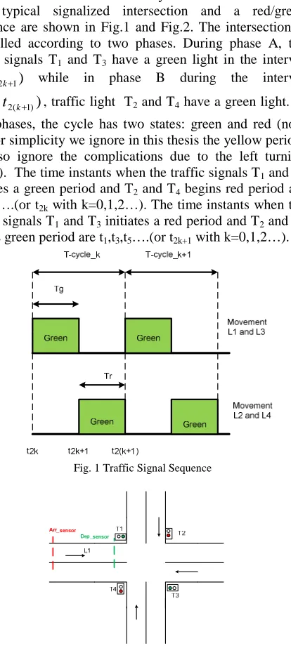
A typical signalized intersection and a red/green sequence are shown in Fig.1 and Fig.2. The intersection is controlled according to two phases. During phase A, the traffic signals T1 and T3 have a green light in the interval

)

,

[

t

_2k

t

_2k+1 while in phase B during the interval

)

,

[

t

_2k+1

t

_2(k+1) , traffic light T2 and T4 have a green light. In

both phases, the cycle has two states: green and red (note that for simplicity we ignore in this thesis the yellow period; we also ignore the complications due to the left turning traffic). The time instants when the traffic signals T1 and T3 initiates a green period and T2 and T4 begins red period are t0,t2,t4….(or t2k with k=0,1,2…). The time instants when the traffic signals T1 and T3 initiates a red period and T2 and T4 begins green period are t1,t3,t5….(or t2k+1 with k=0,1,2…).

Fig. 1 Traffic Signal Sequence

Fig. 2 Intersection with incoming lanes

Notation: Subscript i=1,2,3,4 indicates the number of the approach lane Li, while the Greek character λ or µ indicates that it is an arrival or departure flow. Subscript t indicates the real-time, while tk denotes the starting time of red and

green phases; remember that these flow rates remain constant during an interval t ∈ [tk, tk+1) . Example: the arrival rate of vehicles in traffic movements L1 and L3 in the interval [t2k, t2k+1) are λ1,t_2k and λ3,t_2k and in the interval

[t2k+1,t2(k+1)) are

1 2 , 1tk+

λ and 1 2

, 3tk+

λ

. The departure rate of vehicles in movements L1 and L3 in the interval [t2k, t2k+1) is

k

t2 , 1

µ and

k

t₂

, 3

µ

.

Consequently, one can see that t2k+1-t2k = Tg,k and t2k+2 -t2k+1 = Tr,k, where k is a cycle index. Therefore, Tg,k represents the green time and Tr represents the red time in traffic signal T1 and T3. A cycle length Ck=C is equal to Tg,k+Tr,k, wherein this paper; cycle length is constant.

Formulation of the queue length trajectories can be expressed equivalently as a piecewise affine model. The evolution of the queue length, for traffic signal T1 and T3, in movements L1 and L3 are obtained by:







∈

∈

−

=

+ +

+

]

,

[

,

]

,

[

),

(

1

)

(

2 2 1 2 ,

1 2 2 _

, , ,

k k t

i

k k t

i t i t i i

t

t

t

i

t

t

t

q

dt

dq

λ

µ

λ

(1)

for i=1,3; k=0,1,2…and 1(.) is the indicator function defined as







>

=

otherwise

z

if

z

0

0

1

)

(

1

where

z

=

q

_{i,t_} This indicates that queue-length in

movement i is bigger than zero. Notation t_ in

q

i,t_means

that we consider the value of the queue length just before time t2k+1, something that is well defined because qt is a

piecewise continuous function, with left-hand limits. The relation of the queue length between the time instants t2k and t2k+2 are represented by the following equations:





+

+

+

+ + +

>

−

+

=

+

=

1 2

2 2 1 2

2 2

1 2 1 2 1 2

0

)

(

1

)

(

, , , _

, ,

, ,

,

k

k k k

k

k k k

t

t

t i t i t i t

i t i

t

t t i t

i t i

q

q

q

dt

q

q

µ

λ

λ

(2)

for i=1,3 and k=0,1,2…The equation describing the relationship of the queue length at traffic movement L2 and L4 are obtained in a similar manner and please note that in (1) and (2), the arrival and departure flow rates are nonnegative values, and the queue-lengths will never become negative (but can be equal to 0), thanks to the inclusion of 1(qi,t_) in the equations describing the evolution

of queue lengths.

C. Jump Markov Model

Different from our previous work on traffic control where one assumed that traffic flow is deterministic or using TOD approach, in this work defines the traffic flow rates as stochastic variables. This section describes in detail the complete stochastic hybrid model for one signalized intersection, also called further on the jump Markov model (JMM). In order to express this, we use a mode dependent

AR model for a generic traffic flow rate

k

t

α

(which could represent the arrival flow rate

k

t

λ

or the departure flow rate

k

t

µ

). Remember that the period of the cycle is noted [t2k t2(k+1) ) which consists of green phase and red phase during a period of time when the traffic conditions, also called the mode s of operation of the traffic, remains unchanged, this variable

k

t

α

is modelled by a first-order autoregressive (AR) model:

k k

k t t

t

β

s

γ

s

α

η

α

₊

=

(

)

+

(

)

+

1 (3)

(where

β

(s

)

and

γ

( s

)

are mode-dependent

parameters to be identified, and

,

k

=

1

,

2

,

....

k

t

η

is an

independent identically distributed sequence of zero mean

Gaussian random variables with variance

σ

2

(

s

)

, with

σ

2

(

s

)

also a mode dependent parameter to be identified).

In the traffic flow model introduced in this subsection we consider 2 or 3 different values for the mode of operation

{ }

1

,

2

∈

k

t

s

:

-

=

1

k

t

s

denotes the desirable mode of operation where traffic is flowing freely without too much interference between successive vehicle;

-

=

2

k

t

s

denotes the congested mode where

vehicles hinder each other significantly, and the system operates inefficiently;

This paper assumes that the mode process k

t

s

can be

modelled by a first-order Markov chain, i.e., at each time

t

_k the mode variable

s

i

k

t₋1

=

changes randomly to the value

j

s

k

t

=

with a transition probability Πij=

Prob

(

|

,

,

,

...)

3 2

1 − −

−

=

=

_{k k k}

k t t t

t

j

s

i

s

s

s

which only depends

on the most recent mode (or Markov state)

1

−

k

t

s

, not on states further in the past. Equation (3) with its interpretation

k

t

t

α

α

(

)

=

for

t

∈

[

t

_k

,

t

_k+1

)

, together with the Markov chain

model for the mode k

t

s

, and the queueing model of equation (1-2) provides us with a complete mathematical model of traffic flow. The parameters of this model will be estimated in the next section according to the expectation maximisation (EM) parameter estimation In total there are 10 parameters to be estimated for one single approach lane Li: (a) for each mode

s

∈

{ }

1

,

2

,

the AR model has 3

parameters,

β

(s),

γ

(s

)

and

σ

2

(

s

)

,for total of 6 parameters to be estimated; (b) the transition matrix Πij of the Markov chain describing the mode process has 2 rows of 2 elements,

satisfying the normalization condition



=

∀

=

Π

2 , 1

,

1

j

ij

i

, for

a total of 4 free parameters to be estimated.

The main advantageous of JMM stochastic approach is that the transition matrix does not only determine the ergodic probability but also determine how long the mode stays. This is something that cannot be provided by deterministic model and TOD. The similarity between TOD and deterministic model is weak in accuracy especially in transitions between clusters/modes. While the difference, deterministic approach will be more accurate in the evolution of traffic flow within each cluster compared with TOD which basically is based on averaging the previous daily data.

D. Particle Filtering: State Estimation of Hybrid System

In this part, we use an expectation-maximization technique proposed in our paper [7] to estimate parameters

{

Π

}

=

,

,

,

,

,

2

,

2 2 2 2 1 1

1

γ

σ

β

γ

σ

β

θ

of hybrid stochastic

systems. Please refer to paper [7] for the detailed algorithm and based on those parameters, we use particle filter to estimate

)}

,

(

),

,

(

),

,

(

,

{

}

{

2 2 1 2 1 2 2

2 1, 1,

,

1 k k k k k k

k

k t t t t t t t

t

q

s

s

s

x

λ

λ

µ

+ +

=

as

defined by equation (1), (2) and (3).

A particle filtering (PF) is a Monte Carlo, or simulation based, an algorithm for recursive Bayesian Inference. That is, it approximates the predict-update cycle, and it is very widely used in many applications, including tracking, time-series forecasting, online parameter learning, etc. Please refer paper [12][14] for a detailed description of the PF algorithm for the interested reader.

A number of suggestions have been proposed in order to make the standard PF applicable to the state estimation problem of hybrid processes: interacting multiple model

particle filtering (IMMPF) [11] and observation and transition-based most likely modes tracking particle filter

(OTPF) [9].

In this subsection, we will review the OTPF applied to the jump Markov model of section 4. In this case, one needs to calculate the probability density function (pdf) of the hybrid system

(

,

|

)

k k k t t

t

s

x

p

y

, where

k

t

x

still denotes the

state of the AR models, while

k

t

s

indicates the mode of the system at time tk where s=1,2,…,K. In this subsection, we

focus on the state estimation assuming that AR parameter and TPM are known a priori through EM technique, which is a standard a requirement in the usual applications of the OTPF.

State estimation based on OTPF calculates the

conditional pdf of a hybrid system:

(

,

|

)

k k k t t

t

s

x

p

y

,

}

,

,

0

,

{

j k

t_k

=

y

j

=

…

t

system only follows one mode, it is reasonable to assume

that it is actually only following the most-likely mode k t

sˆ

:

)

|

(

)

|

(

)

,

|

(

)

|

(

)

,

|

(

)

|

(

)

,

(

k k tk k k k k k k k k k k k k k k k t t s t t t t t t t t t t t t t t t

x

p

s

p

s

x

p

s

p

s

x

p

s

p

s

x

p

y

y

y

y

y

y

y

⌢

⌢

⌢

⌢

=

≈

=

(4)

Since

(

|

)

k

k t

t

s

p

⌢

y

is a constant in (4) its effect will be

absorbed in the normalization constant and will not affect the basic PF algorithm.

III.RESULTS AND DISCUSSION

A. Traffic Flow Case: Actual Data

This section focuses on modelling urban traffic flow as indicated in (3), by estimating parameter values based on the EM algorithm of our paper [7],[8] using the data over a time window [0,T] for the experiment layout in city of Jakarta (data courtesy of the Newtel Pvt Ltd). The time-window size is important to define the model that will be used for estimating traffic flow. In this section, for this purpose, we use the above-described data as input for the EM algorithm for 1 day (0 pm–24 am) obtained on 1 September 2012, from the video cameras installed for the operation of the SCATS traffic control system. The data are taken from the area of Thamrin street (data courtesy of the Newtel Pty Ltd.). The aim of the current experiment is to check the practical implementation of our algorithm by:

a) identifying the parameters

{

Π

}

=

,

,

,

2

,

2

,

22

,

2 1 1

1

γ

σ

β

γ

σ

β

θ

of the JMM model (3)

with 2 modes. Based on the actual data and EM technique we find the best estimate value of θ ={0.1325,0.4736,0.0208,0.0895,0.6829,0.067,       8617 . 0 1383 . 0 2131 . 0 7869 .

0 _{}. Parameter θ is used to complete the}

jump Markov model of arrival flow. Based on the model, we use a particle filter as described in the previous section and in [9],[10],[11],[12] to estimate arrival flow. The results in the Fig.3 below shows that the measurement data fits with estimated traffic flow and it means that the JMM with 2 modes and estimating a parameter θ can be classified as a suitable model of the traffic flow.

b) identifying the parameters

{

Π

}

=

,

,

,

,

,

,

,

,

2

,

3 3 3 2 2 2 2 2 1 1

1

γ

σ

β

γ

σ

β

γ

σ

β

θ

of the JMM

model (3) with 3 modes. Based on the actual data and EM technique we find the best estimate value of

θ={0.1621,0.1184,0.0441,0.1065,0.6195,0.0071,0.1431,0.4 897,0.0158,Π}, where

          = ∏ 878 . 0 122 . 0 0 0916 . 0 888 . 0 02 . 0 0 373 . 0 626 . 0

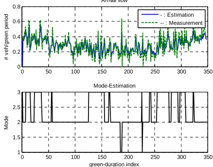
The good fits between the evolution of arrival flow measurements and estimation as depicted in Fig.4 show that the model JMM with 3 modes and parameters θ can be a

good candidate model of traffic flow. By using these parameters, we can characterize the JMM model of the traffic flow in each of the three modes, and the transition probability matrix

Π

. Since for all estimated values we find that |γ| <1, the stationary value Ei(α(t))=βi/(1-γi), where i=1,2 and 3. It is clear from the results of parameter estimation θ and the evolution of modes in Fig.4 that the EM technique is able to identify the modes. The second and third modes have an average value Ei(α(t)) that is almost the same but with different values of the variance. Both modes can be classified as a congestion mode. A value for the variance that is almost doubled is a strong indication that the third mode is a congestion mode with higher uncertainty.

110 120 130 140 150 160 170 180 190 200 0 0.1 0.2 0.3 0.4 0.5 0.6 0.7

Green-duration Index of I-313

# v e h / G re e n p e ri o d Arrival flow -: Estimation .-: Measurement

Fig. 3 Measurement and estimated of arrival flow

By estimating the parameter θ of proposed SHM for the

traffic flow both for arrival and departure flow over the successive cycles of the traffic light, one can define the evolution of queue length by using (2).

0 50 100 150 200 250 300 350 0 0.2 0.4 0.6 0.8 Arrival flow # v e h /g re e n p e ri o d

0 50 100 150 200 250 300 350 1 1.5 2 2.5 3 Mode-Estimation green-duration index M o d e

- : Estimation -- : Measurement

Fig. 4 Evolution of traffic flow and modes

B. Queue Length Case: Synthetic Data

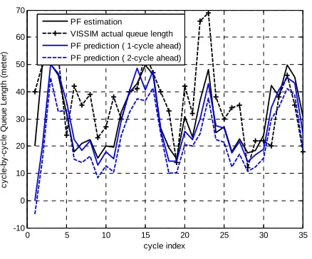
software offers makes it possible to validate our algorithm using the VISSIM traffic micro-simulator. We use VISSIM as a microscopic traffic simulator generating synthetic traffic data implementing a detailed model with the same traffic flow rates as for the hybrid dynamic SHM model introduced in the previous section. The simulated output can be made more realistic by generating the noise as required for realistic representation of traffic irregularity, mode changes. Moreover, VISSIM allows the user to read out data like current traffic flow, and queue length at different locations, data that after adding measurement noise, can be used as the simulated output of real traffic sensors. These synthetic output data ytk simulate the sensor output available for online analysis. The output of such a simulation run provides the noisy data about traffic flow rates under various conditions, for the time intervals corresponding to the cycle of the traffic lights. Hence comparing the queue length obtained via microsimulation with the estimations and predictions obtained via the PF estimator provides a fair and honest way of validating the correctness of the proposed estimator method. In the PF approach, prediction of traffic flow over one or two cycles ahead is performed by using JMM equation (3). Let assume at time tk,

the parameter θ={β,γ,σ2} and also mode k

t

s

has been identified by parameter estimation and based on the

equation (4) and also Πij then the traffic flow rate

α

t_k+1 can

be predicted and so on for the

2

+

k

t

α

. Fig.5 shows that the PF queue length estimator and predictor gives results close to the ”synthetic” VISSIM queue length.

0 5 10 15 20 25 30 35 -10

0 10 20 30 40 50 60 70

cycle index

c

y

c

le

-b

y

-c

y

c

le

Q

u

e

u

e

L

e

n

g

th

(

m

e

te

r)

PF estimation

VISSIM actual queue length PF prediction ( 1-cycle ahead) PF prediction ( 2-cycle ahead)

Fig. 5 Queue length prediction

IV.CONCLUSION

This paper proposed a hybrid dynamic system model as a powerful approach for capturing the complicated dynamics of urban traffic flow, including many sources of uncertainty. The model was appealing as traffic flow conditions can be classified into two or three modes and the switch between these three modes was controlled by a first-order Markov chain. The model was characterized by a set of parameters to be estimated using measured data (e.g., from a video

camera overlooking traffic), and it was shown that a particle filter technique might lead to a useful real-time state estimation algorithm that can be part of a feedback control loop.

The study reported in this paper investigated the proposed approach both by using actual traffic flow data and synthetic data and confirmed its validity by showing that the particle filter based on the identified model provided satisfactory state estimation and correctly captured the random variation of the traffic flow. The proposed hybrid model along with the particle filter estimator will be applied to a paper in preparation for queue length estimators as a crucial part of the synthesis of traffic light control.

ACKNOWLEDGMENT

The first author would like to especially acknowledge to René Boel at Ghent University for deep and helpful discussion. The work of the authors was supported by Science and Technology Development Research Grant 2016, Ministry of Research and Higher Education, Indonesia.

REFERENCES

[1] K. Aboudolas and N. Geroliminis, ”Perimeter and boundary flow control in multi-reservoir heterogeneous networks,” Transportation

Research Part B, vol. 55, pp. 265-281, 2013.

[2] N. Geroliminis, J. Haddad, and M. Ramezani, ”Optimal Perimeter Control for Two Urban Regions With Macroscopic Fundamental Diagrams: A Model Predictive Approach,” IEEE Transaction on

Intelligent Transportation Systems, vol. 14, issue 1, March 2013.

[3] C.F. Daganzo, “Urban gridlock: Macroscopic modeling and mitigation approaches,” Transp. Res. B: Methodol., vol. 41, no. 1, pp. 49–62, Jan. 2007.

[4] H.Y. Sutarto, et.al., ”Hybrid Petri net model of a traffic intersection in a urban network,” IEEE Multi-conference on Systems and Control,

Yokohama, Japan, sept 2010.

[5] M. Zaky, D.G. Airulla, E.Joelianto, and H.Y. Sutarto, ”Urban Traffic Simulation Using SUMO Open Source Tools,”

Internetworking Indonesia Journal, vol. 9, no. 1, pp. 83-88, 2017.

[6] J. Haddad, B. de Schutter, D. Mahalel and P.O. Gutman, ”Steady-State and N-stages Control for Isolated Controlled Intersections,”

Proceeding American Control Conference, 2009, St. Louis, MO,

USA, June 2009, pp. 2843-2848.

[7] H.Y. Sutarto, R. Boel, and E. Joelianto ”EM-Parameter estimation for stochastic hybrid model applied to urban traffic flow estimation,”

IET Control Theory and Applications, vol. 9, Issue 11, 2015.

[8] H.Y. Sutarto and E. Joelianto, ”Expectation-Maximization Based Parameter Identification for HMM of Urban Traffic Flow,” Int. J.

Appl. Math. Stat., vol. 53, Issue No.2, 2015.

[9] S. Tafazoli and X. Sun, ”Hybrid system state tracking and fault detection using particle filters,” IEEE Trans. Control Syst. Technol., vol.14(6), pp. 1078–1087, 2006.

[10] Y. Xue and T. Runolfsson, ”Efficient estimation of hybrid systems with application to tracking,” International Journal of Systems

Science, DOI:10.1080/00207721.2011.5666-41, 2011.

[11] H.A.P. Blom and E.A. Bloem, ”Exact bayesian and particle filtering of stochastic hybrid system,” IEEE Transactions on Aerospace and

Electronic Systems, vol. 43(1), pp. 55-70, 2007.

[12] H.Y. Sutarto, E. Joelianto, and T.S. Sumardi, ”Estimation and Prediction of road traffic flow using particle filter for real-time traffic control,” 2nd IEEE Conference on Control, Systems &

Industrial Informatics, 2013.

[13] W. Glover and J. Lygeros, ”A Stochastic Hybrid Model for Air Traffic Control Simulation,” Hybrid Systems: Computation and

Control Volume 2993 of the series Lecture Notes in Computer Science, pp. 372-386, 2004.