The properties of a stochastic model for two competing species

Patron: Her Majesty The Queen Rothamsted Research Harpenden, Herts, AL5 2JQ Telephone: +44 (0)1582 763133 Web: http://www.rothamsted.ac.uk/

Rothamsted Research is a Company Limited by Guarantee Registered Office: as above. Registered in England No. 2393175. Registered Charity No. 802038. VAT No. 197 4201 51. Founded in 1843 by John Bennet Lawes.

Rothamsted Repository Download

A - Papers appearing in refereed journals

Leslie, P. H. and Gower, J. C. 1958. The properties of a stochastic model

for two competing species. Biometrika. 45 (3-4), pp. 316-330.

The publisher's version can be accessed at:

•

https://dx.doi.org/10.1093/biomet/45.3-4.316

The output can be accessed at:

https://repository.rothamsted.ac.uk/item/8w1w7

.

© Please contact library@rothamsted.ac.uk for copyright queries.

[ 316 ]

THE PROPERTIES OF A STOCHASTIC MODEL

FOR TWO COMPETING SPECIES

B Y P. H. LESLIE AND J. C. GOWER

Bureau of Animal Population, Department of Zoological Field Studies, Oxford and Rothamsted Experimental Station

1. INTRODUCTION

A stochastic model for studying the properties of certain biological systems by numerical methods has been described in an earlier paper (Leslie, 1958), to which reference should be made for the full details of its development. Two varieties of this model for the case of two competing species have been programmed for the Elliot-N.R.D.C. 401 computer in the Statistical Department of Rothamsted Experimental Station, and some of the results obtained are given in the following paper.

2. THE MODELS USED

Suppose that two species Sx and S2 are competing together in a limited environment, and

that their populations consist of N^t) and N2(t) individuals at time t. Then it is assumed that

the expected balance of births and deaths in the two populations during the discrete interval of time t to t +1 is denned by the deterministic model,

v_ Ax

(X 1) where the functions

= l+o1JVr1(0+A#2(0,l , - a

1 (a1; a2, plt p2,

and the constants loge A.x = ^i,logeA2 = r2 are the intrinsic rates of increase of the two species.

This system will have a stationary state when ql = X1 and q2 = A2, or when

T -l ~ x ~

If we define the ratios x *-—— = y, ^-i£? = x,

then, in the deterministic model, the following four possibilities arise:

x<y<\. Stable stationary state (both Sx and S2 persist).

1 < y < x. Unstable stationary state (either Sx or S2 persists, depending on the initial

state of the system).

y < 1, x > y. Sx persists and S2 disappears from the system. y > 1, x < y. S2 persists and Sx disappears from the system.

P. H. LESLIE AND J. C. GOWER 317

By a suitable choice of the parameters in (1-1) we thus can construct a numerical system which will fall into one or other of these four categories.

An innumerable variety of different stochastic models can be imagined which will have the same deterministic equivalent, depending on the assumptions made as to the birth-rate and death-rate functions for the two populations (cf. Bartlett, 1957). But these possibilities can be regarded as falling between the extreme cases of either the birth-rate or the death-rate of each species remaining constant. In order to study the qualitative properties of this type of system, we may work in terms of these two limits, and we shall consider, therefore, the following two models.

Model I, in which it is assumed that the birth-rate of each species remains constant

We have in (1-1) the constant

Aa = e'« = e6«-<*« (a = 1 , 2 ) , (1-3) where the intrinsic rate of increase ra is the difference between a birth-rate ba and a

death-rate da(ba > da). Since the birth-rate of each species is assumed to remain constant, we have

for the discrete interval of time ttot+1,

log, IKkaim = log, Aa(«) = ba- da(t) (a = 1,2),

where the death-rate da(t) is a function of Nx(t) and N2(t), and is regarded as remaining

constant during the interval. Then, from the standard theory of simple 'birth' and 'death' processes, it may be shown that if we adopt for our two hypothetical species values of A,

b and d in (1-3) such as

X b d

2-0 1-0083 0-3151]

2-5 1-0308 0-1145] ^ '4'

then in the stochastic model, we may take

where Aa(£) is defined in (1-1). In order to simplify matters in practice, we assume as an approximation that Na{t +1) is distributed normally with /ia and «r| given by (1-5),

attri-buting all negative values to Na(t +1) = 0. Thus, given N±(t) and N2(t) at time t, Nx(t + 1) and N2(t+ 1) can be calculated with the help of a pair of random normal deviates, and the

pro-cesses can then be continued with the resulting values.

Model II, in which it is assumed that the death-rate of each species remains constant

In this case we now have in (1-1) for the interval of time ttot+1,

log

IKIUm = log

K(t) = bjt) -d

(a=l, 2),

where ba (t) for the particular species is a function of N^t) and N2(t), and the death-rate da

remains constant. Because no meaning can be attached to a negative birth-rate, we there-fore have to define

Ao(«) =

since ba(t) = 0, when qa{t) = eb*; and

Then, provided we adopt the same values of A, b and d as given in (1-4), we have

E[Na(t + l)] = \a(t)Na(t) (Aa>,

(a = 1 , 2 ) I (1-6)

= (1 - e-ta) E[Na(t + 1 ) ] (qa{t);

where the functions /[Ao(£)] in the expression for the variance, for the two values of A, are given by the linear relationships,

A = 2-5: /[A(<)] = - 0-87 + 1-10 A(*), A = 2-0: f[\(t)] = - 0-66 + 1-29A(<).

As before, we assume that given N^t) and N2(t) at time t, then Nt(t + 1) and N2(t + 1) a r e distributed normally with these means and variances.

3. PROGRAMMING OF THE MODELS

The programme was so arranged that the constants alt a2, filt fi2, A,, A2 were read into the computer at the beginning of each run, together with a pair of random numbers and the initial population size for each species. It was thus possible to vary these parameters very easily and so study the models under different conditions. The random numbers were re-quired to start a process for producing pseudo-random numbers and eventually random normal deviates; the possibility of using existing tables of random numbers was excluded since about 40,000 numbers might be required for each initial point estimated. The method adopted was as follows:

(i) Choose p and x' at random, e.g. from a table of random numbers. (ii) Replace x' by x, the closest number to x' such that x = 5 (mod 8). (iii) Form successively the numbers pxn mod (2*), n = 1,2,3,....

Under these conditions it can be shown (the proof resting on a theorem of Euler) that the numbers so formed form a repeating cycle of 2k~2 different numbers. In fact the successive powers of a; are all the-2*~2 numbers (mod 2k) whose last two binary digits are 01, where for the Elliot 401 computer k is taken to be 32. By choosing different values of p the sequence may be generated in different orders. The main advantage of this over other methods advocated for generating pseudo-random numbers is that it is impossible to get into a closed loop generating zero or the same few numbers over and over again. Tests for various types of departure from randomness for this method have been reported in the literature (Foster, 1954; Taussky & Todd, 1956), and it has generally been found to be satisfactory. Con-sequently, only a very simple test, which may be regarded as a form of quality control, was incorporated in the programme.

Random normal deviates were produced by summing twelve variates (uniform in the range — £ ^ x ^ £) produced by the above method. Such a deviate will have zero mean and unit variance. A running total was kept of all deviates of magnitude greater than two, together with the total number of deviates used. These deviates were not rejected since otherwise an undesirable bias would have been introduced into the process.

For each pair of initial population values in the case of a system with an unstable stationary state, the programme was arranged to run through sixty representations of the population

P. H. LESLIE AND J. C. GO WEB 319

growth, stopping when one or other of the species had become zero. For each representation the number of units of time required to reach extinction and the particular species which had vanished were recorded in the machine. After all sixty trials the probability that species S1

survived and its standard deviation were printed, together with the distribution of the time to extinction for each species and the observed and expected number of normal deviates used of magnitude greater than two. (These ' normal' deviates are in fact the sum of twelve uniform variates, as explained above, so that the appropriate percentage point is 0-04455 as opposed to 0-04550 for the normal distribution (Hall, 1927).)

The programmes for the two models differed only in the evaluation of the expression for var [N{t + 1)], so that the modifications required were almost trivial.

4. T H E PROPERTIES OF A SYSTEM WITH AN UNSTABLE STATIONARY STATE

When the deterministic model has an unstable stationary state, the final outcome of the interaction depends on the initial state of the system. Consequently, in the stochastic model, it might be expected that random variations, more particularly in the early stages of population growth, could be an important factor in deciding which of the two species would survive (Bartlett, 1957).

In order to investigate this point, the numerical values of the parameters in (1-1) were taken as

Ax = 2-5: qx = 1 + 0-0030 Nx + 0-0105 N2,

A2 = 2-0: q2 = 1 + 0-0025iV2 + 0-0050^,

which, from (1-2), give an unstable stationary state with Lx = 150 and L2 = 100.

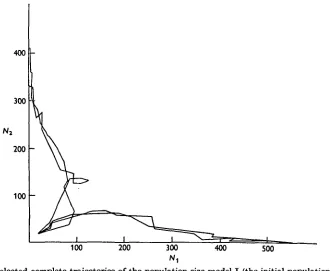
Suppose, for example, that in the deterministic model we take Nx(0) = N2(0) = 20, then

by a repeated application of equations (1 • 1) it appears that given these initial conditions, the species S2 will always survive and S1 will disappear from the system. (Given other initial

conditions, of course, this would not necessarily be the case.) But in both types of stochastic model, I and II, it was found that with these same initial conditions, the processes sometimes went in one direction and sometimes in the other. A few typical (Nlt N2) trajectories for

model I are given in Fig. 1. It was clear from these preliminary results that at any point on the (NltN2) plane there would be a probability, O^p^l, that ultimately the species Sx

would survive and S2 disappear from the system. It was of interest, therefore, to determine

the contour lines of p for the two extreme types of stochastic model.

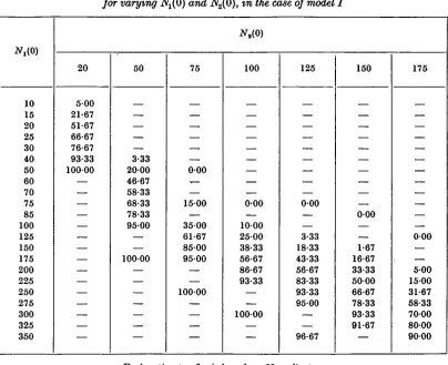
We give in Table 1 the estimated values of p, in the case of model I, for a number of points on the plane, each of these estimates being based on 60 replicates. These points can be re-garded either as the initial conditions at t = 0 of some particular system, or as the conditions at time t of a system which started at some previous time t — a. By a suitable change in the origin of the time scale for the latter, the two cases become equivalent. The general pattern of the distribution of p can be seen from the entries in this table. For a fixed value of N2(0), p steadily increases with increasing i^(0) until it becomes 100 %. Thus, if the trajectory of

a particular replicate were to reach the region where p ~ 1, this means that the species Sx is

almost certain to survive, and that the chance of any reversal in the trend is negligibly small. Conversely, a trajectory reaching the region where p ~ 0 means that the species S2 is almost

certain to survive.

In order to map the contour lines of p, we made use of the empirical observation that for each value of N2(0) in Table 1, the probit of p was linearly related to log N^O). These probit

lines were calculated in the usual way, and in each case the x2 goodness of fit test was

satis-factory. The only feature of these lines which should be mentioned is that the slopes steadily increased with increasing iV3(0); in other words, a probit plane could not be fitted to the results given in Table 1. The contour lines foip = 95, 50 and 5 % which were calculated from these regressions of probit p on log Nt(0) are given in Fig. 2, the irregularities in the figure

being due to the sampling errors involved in the estimates. The spread of the contour lines is fan-shaped, and in this numerical system the 50 % line passes through the unstable equili-brium point, Lx = 15O,L2 = 100. (The estimated 50% point for N2(0) = 100wasi^(0) = 155, with a fiducial range (P = 0-95) of 149-162.) However, there is no reason to think that this would necessarily be true for all systems with an unstable stationary state.

Fig. 1. Selected complete trajectories of the population size model I (the initial population in each case is Nt = Ns = 20).

The results of a similar series of calculations using model II are given in Table 2. For relatively small values of the initial numbers the probability p appears to be much the same in the two models (cf. the estimates for Nz(0) = 20 and variable N^O) in Tables 1 and 2); but

in model II, as iV2(0) increased in magnitude, the slopes of the probit lines became steadily greater than those for model I, leading to a narrower band of probabilities lying between

p ~ 0 and p~\. This is shown in the comparable graph of the 95, 50 and 5 % contour lines

of p, given in Fig. 3. This smaller spread is presumably due to the smaller variance of this model.*

* That the smaller spread of the contour lines in Fig. 3, compared with that in Fig. 2, is due to the smaller variance of model II, was confirmed accidentally by a set of calculations using model I in which, through an error in programming, it was assumed that var [.No{< + 1)] for each species was equal to 0-5 E [Na(t+ 1)], instead of the correct approximation var [Na(t+ 1)] = 2E [Na(t+ 1)]. Exactly the

same pattern of contour lines emerged as in Fig. 2, but the fan-shaped spread was very much less.

P. H. LESLIE AND J. C. GOWER 321

From the fitting of the probit regression lines for each fixed value of N2(0) in Tables 1 and 2,

the estimated 50 % points for Nt(0) were the same in the two models, apart from errors of

random sampling, up to N2(0) = 125; but for N2(Q) = 150 and 175 they were significantly

less in model I I than in model I, leading to the curvature of the contour lines which can be seen in Fig. 3. The explanation of this difference between the two models appears to be that

Table 1. Estimates of the probability p (%) that the species St will survive, for varying N^O) and N2(0), in the case of model I

10 15 20 25 30 40 50 60 70 75 85 100 125 150 175 200 225 250 275 300 325 350 20 500 21-67 51-67 66-67 76-67 93-33 10000 — — — — — — — — 50 — — 3-33 2000 46-67 58-33 68-33 78-33 9500 — 10000 — — — — — 75 — — — 000 -, 1500 — 3500 61-67 85-00 9500 — — 10000 — — 100 — — — 000 1000 2500 38-33 56-67 86-67 93-33 — — 10000 — 125 — — — — 000 — 3-33 18-33 43-33 56-67 83-33 93-33 9500 96-67 150 — — — 000 — — 1-67 16-67 33-33 5000 66-67 78-33 93-33 91-67 — 175 — — — — — — — 000 500 1500 31-67 58-33 7000 8000 9000

Each estimate of p is based on 60 replicates.

in this particular numerical system the processes may be involved with the discontinuities in model II, which are due to the restriction that the birth-rate of each species becomes zero when<7a = e6«(a = 1,2). When qa<eb°the expected numbers E[Na(t+ 1)] are the same in both

models for given N^t) and N2(t); but if this is not the case, then the expectations are different.

To take as an example a typical point in this region of the plane, suppose that JV^O) = 225 and N2(0) = 175. Then, from (1-1) and (1-4) we have

qx = 3-5125 > e"i = 2-8033, q2 = 2-5625 < e*« = 2-7409.

Hence from (1-5) and (1-6) the expected numbers aU = lare^[iVi(l)] = 201,E[N2(l)] = 137

in the case of model II, and ElN^l)] = 16O,E[N2(1)] = 137 in model I. Thus, the trajectories

Table 2. Estimates of the probability p (%) that the species /Sx will survive,

for varying ^ ( 0 ) and N2(0), in the case of model II

NJO) 10 15 20 25 30 40 50 60 70 75 100 110 125 150 175 190 200 220 225 250 275 300 20 6-67 18-33 58-33 7000 8000 9500 10000 — — — — — — — — — — — — — — 50 000 1-67 11-67 31-67 58-33 68-33 10000 — — — — — — 75 — — — 000 500 3000 68-33 91-67 10000 — — 100 — — — — 000 — 1000 5500 91-67* 99-17* 10000 10000 10000 125 — — — — 000 500 16-67 5500 7000 10000 — 150 — — — — — — 000 3-33 2500 83-33 98-33 10000 10000 175 — — — — — — — — — — — 000 — 8-89f 41-67 58-33 98-33 10000

* Estimate based on 120 replicates, f Estimate based on 180 replicates. All other estimates based on 60 replicates.

200 180 160 140 120 100 80 60 40 20

i i l l I j I

20 40 60 80 100120140160180 200220240260 280 300320 340360 380

Fig. 2. Contour lines for percentage probability that <S, survives and St disappears, model I.

P. H. LESLIE AND J. C. GOWEB 323

for the two models start off by following, on the average, different paths, and the divergence between them becomes greater with increasing time. From the direction of the difference between the mean paths for given N2 (e.g. JE?[2^(1)] for I I > ElN^l)] for 11 E[N2(l)] = 137),

we should expect, therefore, that the probability p associated with these initial conditions would be greater in the case of model I I than in model I. Since the majority of the points tested for fixed N2(0) = 150 and 175 fell in the same region where gx > e6i, q2 < e*«, there would

tend to be a greater probability of the species Sx surviving in the constant death-rate type of

model for such initial conditions of this numerical system.

200

180

160

140

120

100

80

60

40

20

5% 50% 95%

1

20 40 60 80TOO 120 140160 180 200 220 240 260 280

Fig. 3. Contour lines for percentage probability that <SX survives and <S2 disappears, model II.

The difference between the two models for these rather extreme initial states of the system in relation to the unstable stationary point is possibly of less interest, however, than the agreement between them for the remaining points tested. It can be seen from Figs. 2 and 3 that, broadly speaking, the general pattern of the contour lines of p in the remaining regions of the plane is very similar for the two models, apart from the degree of spread, and we can infer that the results for all the other possible types of stochastic model which have this same deterministic equivalent would fall somewhere in between the results for these two limiting cases.

5. RESULTS FOR A SYSTEM WITH A STABLE STATIONARY STATE

As a contrast to this type of system, suppose we take the case of a stable stationary state with Lx= 150 and L2 = 100, for example if in (1-1) we have

Ai = 2-5: ft = 1 +0-00800^+ 0-003002V2,

A2 = 2-0: = 1+0-00625^ + 0-002502^.

Two realizations were calculated for this system using model I, because of the saving of machine time in the case of this model, and also because of its greater variance. Taking the initial state of the system as i^(0) = iV2(0) = 20, the values of-ZV^) and N2(t) were printed off

at each step in the calculations, the first realization being computed up to t = 149, and the second up to t = 70.

These processes rapidly approached their equilibrium levels, in the region of which they then continued to fluctuate in an irregular fashion. As an illustration, the results for the second realization are given in Fig. 4, neglecting the first six steps in the calculation during

N(t) 22Sr 200 175 150 125 100 75 50 25

10 20 30 40 50 60 70

Time

Fig. 4. Fluctuations around t h e stable stationary state in the case of the second replicate. , species S± (equilibrium level AT1=150); , species S2 (equilibrium level

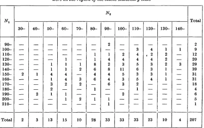
Table 3. Frequency distribution of the observed Nx and N2 when the processes

were in the region of the stable stationary state

90- 100- 110- 120- 130- 140- 150- 160- 170- 180- 190- 200- 210-Total 30-2 2 40-1 2 3 50-1 1 4 1 3 2 1 13 60-1 1 1 4 4 2 1 1 15 70-1 2 3 2 2 10 80-1 1 8 6 4 6 1 1 28 90-2 1 4 2 8 4 4 6 1 1 33 100-2 4 3 11 5 3 3 2 33 110-3 4 4 5 6 3 5 2 1 33 120-4 . 2 4 3 3 3 4 23 130-1 2 2 2 1 1 1 10 140-1 3 4 Total 2 9 12 20 29 39 31 31 18 4 6 5 1 207

P. H. LESLIE AND J. C. GOWER 325

which time an approach was being made to the steady state, Lx — 150, L2 = 100. It will be

seen that although these processes fluctuate around the latter, there is at times a tendency in both cases for a drift to occur away from this region. Thus, in Fig. 4, the numbers of the second species, after fluctuating somewhat above the equilibrium level from t = 20 until about t = 35, then started a slow drift towards the base-line, but later recovered so that at the time the calculations were stopped, the numbers of this species had again returned to the region of the steady state. During this time the numbers of the first species tended to drift in the opposite direction. The same phenomenon, in a varying degree, was also apparent in the results for the first realization, and most probably it is associated with the negative correlation which exists between the numbers of the two species.

We give in Table 3 the observed bivariate distribution of Nx and N2 for the combined data

for the two realizations in the region of the stationary state. From this table we have # ! = 148-3 and^2 =97-2; while var(iV^) = 553-8,var(iV2) = 570-3 and c o v ^ , . ^ ) = -243-4. The type of distribution seems to be approximately normal in form. Thus, if we calculate the expected marginal distributions from the given estimates of the means and variances, we have:

< 9 0 9 0 - 100- 110- 120- 130- 140- 150- 160- 170- 180- 190- 200- 210->220 1-4 2-8 6-6 130 21-3 29-8 34-6 33-3 27-3 18-8 10-2 5 0 2 0 0-7 0-2 Total Expected S-10-8

- 7 - 9

207-0 Observed 207 N, <30 30- 40- 50- 60- 70- 80- 90- 100- 110- 120- 130- 140- 150->160 Expected r12-3 ^7-6 2070 Observed

• 1 8

1

is]

5}

o

For the marginal distribution of Nv we have x2 = 7"3 f °r 7d.f., a perfectly reasonable value to obtain; while for the distribution of N2, x2 = 1 5 - 1 (7<i.f.), a somewhat excessive value which is due very largely to the deficiency of the observed values in the N2 = 70 — 79

class.

I t is of interest to compare the variances of these observed fluctuations in the region of the stationary state with those expected on the theory of small fluctuations for the discrete time model used here.* This model may be written as

Na(t+l)=fa(N1,N2,t) + Za(t+l) (a =1,2),

* We are indebted to Prof. M. S. Bartlett for pointing out to us the following method of

deter-mining the theoretical variances and covariance for the discrete time model.

2i Biom. 45

where the first term is the deterministic part of the process given by (1-1), and the

Za(t+l),(a = 1,2), are independent normal variables with zero means and variances,

in the case when it is assumed that the birth-rate of each species remains constant,

<r2(Za) ~ 2E[Na(t +1)]. In the region of the stationary state

= Na(t+l)-La,

cov (Nt, N2) = cov = E{(ft - LJ (/2 - L2)}.

Hence we have the set of equations for determining the variances and covariance of Nt and N2 when the fluctuations are regarded as small,

2 _ / 3 /x\2 2 9/ 3 / i \ / 3 / i \ /d/i\2 - •

cr% =

cov =

which are to be evaluated for Na = La. Thus, to take the first species as an example, we have

from

Jl 1

(L\

J-lh

\dNjLlL, A, '

and similar expressions in terms of A2, <*2, A a nd L2 from the function/2 for the second species. Given the numerical values of the parameters in the present example, the equations are

O7296cr? + 0-1872 cov -O0324o| = 300,

-0-015625o-f + 0-171875cov + 0-52734375cri = 200,

0-065<rf + 0-62 cov + 0-12375cr| = 0,

whence cr\ = 465-5, a\ = 437-4 and cov = — 136-1. These expected variances and co-variance are less than those actually observed, viz. var (Nj) = 553-8, var(2V2) = 570-3 and cov (Nv N2) = — 243-4; but, apart from the question of the sampling errors associated with

the observed values, the agreement seems to be reasonable when we consider that the expected values are based on the theory of small fluctuations, and so cannot be exactly correct.

I t is perhaps worth noting that if we were to derive the theoretical variances from the type of continuous time model suggested by Bartlett (1955, 1957; cf. also Whittle, 1957) for studying the properties of such stochastic processes in the region of the stationary state, the discrepancy between expected and observed would become much greater. Thus, for a small interval of time St, the equivalent continuous time model for two competing species may be written,

8b\ = ( r ^ - a,N* - k.a.N.N^St + SY1 - 8ZV |

8N2=(r2N2-a2Nl-k2a2N1N2)St + 8Y2-SZ2J

P. H. LESLIE AND J. C. GOWER 327

where SYt, SZ{(i = 1 , 2 ) are independent, modified, Poisson variables with zero means, and

variances, in the case when it is assumed that the birth-rate of each species remains constant,

var (SYt) = b{ Nt St, (i = 1,2)

var (SZi) = (di Nt + af 2VJ + fc, at Nt N2) St.

In the region of the stationary state suppose that Nt = Lt(l +ut) (i = 1,2), then for small u we have from (5-1) the linear stochastic system,

8ux = -a^L^u^ + k^L2u2) St + Si, \

Su2= —

where, for the constant birth-rate type of model, 8E, and 8<fi have variances (2bJL1) St and (2b2IL2)St, respectively. Forming the equations ^ + 8^ and u2 + Su2 from (5-2), we obtain

by squaring, taking the cross-product and averaging the following expressions for the variances and covariance {cr\, a\ and cr12) of % and u2. If we write b1l(a1L1) = X1 and

b2l(a2L2) = X2, then

\ = X1 - kxL2<rX2,

2 2 x

[

.

while the covariance is given by

The values of Lx and L2 are the same in both types of model, while the relationship between

the remaining parameters, in terms of those for the discrete time model, is given by o< = a-i loge A J ^ — 1) and kt = fi^a^i = 1, 2). Since in this particular numerical system bx~b2~\, we have from (5-3), expressing these variances and covariance in the form

var(i^) = ifvar(iti), a\ = 242-1, <r\ = 270-7 and cov = -99-8. Thus it is evident that the theoretical variances of small fluctuations about the steady state are smaller for the con-tinuous time model than for the discrete case.*

It appears, then, that in a system of two competing species with a stable stationary state, the number of individuals over a relatively long period of time settles down to a type of distribution which is approximately normal in form, but with a degree of variation which may be greater than that expected for small deviations about the stable state. This greater degree of variation about the equilibrium level can only lead to an increased chance of random extinction of one or other of the two species.

No calculations were carried out for this system using model II, but it is quite clear that because of the smaller variance of this model, there would have been a smaller degree of variation about the steady state (cf. the results for a logistic process using these two types

* This point also arises in regard to some comparisons which have been made (Leslie, 1958) between the theoretical and observed variances of a number of logistic processes fluctuating in the region of the upper asymptote. A number of replicates were observed over a relatively short period of time, and the estimated variances were based essentially on the pooled 'Within replicates' mean squares. These variances were somewhat greater than those expected from the continuous time model. It appears now that a better agreement would have been obtained if the observed variances had been based on the 'Total' sums of squares and the theoretical variances had been calculated for the discrete time model. For a logistic process these theoretical variances are given by <r2 = 2bKA2/(A2 — 1), when the birth-rate remains constant, and by a2 = 2dKA2/(A2 — 1) when the death-rate remains constant, where in each case K is the upper asymptote in numbers. However, any revision of the estimates given (Leslie, 1958, § 8) would not affect the principal conclusions, namely that in the particular processes studied, the chance of extinction was negligible for any given time interval.

of stochastic model (Leslie, 1958, §8)). Other things being equal, therefore, the chances of random extinction would be less for the second type of model, in which it is assumed that the death-rate of each species remains constant.

6. WHEN ONE SPECIES ALWAYS PEBSISTS

The question remains as to the effect of random fluctuations in the other possibilities which arise in the deterministic model. Thus, if in (1-2) we put

y, _a-tCto

then when y^l,x>y, the species Sx will always persist and S2 will disappear from the

system. When y> 1, x>y, we have the case of the unstable stationary state, and in the deterministic model there is a sharp demarcation between these possibilities when y = 1. In the stochastic model, however, these demarcations must be interpreted more liberally. For instance, if we take the parameters of the system to be

Ax = 2-5: qx = 1 + 0-003001^ + 0-00375iV2, A2 = 2-0: q2 = 1 + 0-002501^ + 0-00500iVi,

then y = 1, x = 2-5, and there is an unstable stationary state with Lx = 0, L2 = 400. In the

case of the deterministic model, the species S1 would always persist, whatever the initial

conditions of the system; but, in the stochastic model, although the probability of the species Sx persisting will be p ~ 1 over most of the (Nv N2) plane, there is still a region where

there is a non-zero probability q = 1 — p that the outcome of the interaction will be reversed. For instance, the following were the estimates of p(%), based in each case on 60 replicates, for the stated values of Nx(0) and iV2(0) in a system with the above parameters, using model I.

Vallies of p (%)

N . Nt(0)

25 50 100

150

98-33 10000 10000

200

95-00 98-33 10000

350

81-67 93-33 10000

400

6000 9000 10000

These results for the borderline case suggest that by making progressive changes in the assumed values of the parameters, it would not be difficult to arrive at a system with y < 1,

x > y, in which the properties of the deterministic model would be changed in no way by

random variations. Similarly, for the case of y > 1, x < y, which in the deterministic model means that the species S2 will always persist.

7. CONCLUSIONS

We may conclude from the results of these experiments that the most important difference between the properties of this stochastic model and its deterministic equivalent is in the case of a system with an unstable stationary state. In the deterministic model this implies that

P. H. LESLIE AND J. C. GOWEB 329

the outcome will depend on the initial state of the system, and that for any given state the particular outcome is then certain to occur. In the stochastic model, however, there is associated with the state of this type of system at any time t, a probability p that ultimately one of the species will survive and the other become extinct, and a probability q = 1 — p that the outcome of the interaction will be reversed.

This feature of the stochastic model is qualitatively very similar to the phenomenon observed by Park (1954) in competing populations of the flour beetles, Tribolium castaneum and T. confusum. The initial conditions adopted in his original experiments (2$, 2$ adults of each species) were the same for all replicates, and batches of replicates were observed under six different combinations of temperature and relative humidity. In four of his physical treatments, T. castaneum survived in a certain proportion p of the replicates, and T.

con-fusum survived in the remaining q = 1 — p, the value of p varying according to treatment

(Park, 1954, table 12, treatments II-V). By plotting the trajectories of the individual replicates for these four treatments, Neyman, Park & Scott (1956) were able, in each case, to divide the (NX,N2) plane empirically into three zones. The two outer of these were

' determinate', since it appeared that if the trajectory of a replicate reached one or other of these zones, only one consequence was then possible, while in between there was an 'indeterminate' zone in which the process might still go either in one direction or the other, though not with an equal probability. Their figures for these zones (Neyman et al. p. 58) show a very similar type of fan-shaped pattern to the graphs of the contour hnes oip, which we have given here in Figs. 2 and 3. A further noteworthy point is the relative consistency of the observed values of p in different experiments with these species, when the populations were initiated with the same number of individuals and kept under similar physical condi-tions (Park & Lloyd, 1955, table 1). In a more recent paper, Park (1957) has examined the relation of the initial numbers to the competitive outcome in populations of these species kept at 34° C., 70% R.H., conditions under which T. castaneum always won and T. confusum was eliminated in his original series of experiments. The results were that out of five different combinations of initial numbers (in terms of eggs) at t = 0, T. castaneum still won in every replicate for four of the combinations; but in the remaining one, the outcome was reversed in some cases, T. confusum winning in five out of the fourteen replicates observed. Thus, the same phenomenon was realized experimentally when the initial conditions of the system were varied.

Clearly, there is a close analogy between the results observed in these experimental populations and the qualitative properties of this model for two competing species, when the stationary state is unstable. But this analogy cannot be taken as direct evidence that the phenomena observed by Park were due to the existence of this type of stationary state in his competitive systems: it can only be regarded as suggestive. In order to decide whether or not this was the case, some quantitative comparisons between the theoretical model and the observed data would be necessary, and for this the type of model used here is of much too simple a form. In its development we have neglected the effect of a changing age distribution on population growth, and factors such as the mutual cannibalism of eggs and pupae by certain age groups, which are known to occur in the case of Tribolium and which necessarily must have an important effect on the growth in numbers and the interaction between these two species. Nevertheless, the results for this simple stochastic model indicate some of the possibilities which may also arise in the case of the more complex models for this type of interaction.

REFERENCES

BARTLETT, M. S. (1955). Deterministic and stochastic models for recurrent epidemics. Proc. Third

Berkeley Symposium on Mathematical Statistics and Probability, 4, 81-109. University of California

Press.

BABTLETT, M. S. (1957). On theoretical models for competitive and predatory biological systems.

Biometrika, 44, 27-42.

FOSTER, F. G. (1954). Contribution to discussion on Symposium on Monte Carlo Methods. J.R.

Statist. Soc. B, 16, 23-75.

HALL, P. (1927). The distribution of means for samples of size N drawn from a population in which the variate takes values between 0 and 1, all such values being equally probable. Biometrika, 19, 240-5.

LESLIE, P. H. (1958). A stochastic model for studying the properties of certain biological systems by numerical methods. Biometrika, 45, 16-31.

NEYMAN, J., PARK, T. & SCOTT, E. L. (1956). Struggle for existence. The Tribolium model: biological and statistical aspects. Proc. Third Berkeley Symposium on Mathematical Statistics and

Pro-bability, 4, 41-79. University of California Press.

PARK, T. (1954). Experimental studies of interspecies competition. II. Temperature, humidity, and competition in two species of Tribolium. Physiol. Zob'l. 27, 177-238.

PARK, T. (1957). Experimental studies of interspecies competition. III. Relation of initial species proportion to competitive outcome in populations of Tribolium. Physiol. Zob'l. 30, 22-40.

PARK, T. & LLOYD, M. (1955). Natural selection and the outcome of competition. Amer. Nat. 89, 235-40.

TAUSSKY, O. & TODD, J. (1956). Generation and Testing of Pseudo-Random Numbers. Symposium on Monte Carlo Methods. (H. A. Meyer, ed.). New York: J. Wiley and Sons.

WHITTLE, P. (1957). On the use of the normal approximation in the treatment of stochastic processes.

J.R. Statist. Soc. B, 19, 268-81.