DEMOGRAPHIC RESEARCH
A peer-reviewed, open-access journal of population sciences
DEMOGRAPHIC RESEARCH
VOLUME 30, ARTICLE 49, PAGES 1397–1404
PUBLISHED 6 MAY 2014
http://www.demographic-research.org/Volumes/Vol30/49/ DOI: 10.4054/DemRes.2014.30.49
Formal Relationship 21
Entropy of the Gompertz-Makeham mortality
model
Tomasz F. Wrycza
c
2014 Tomasz F. Wrycza.
Table of Contents
1. Relationship 1398
2. Proof 1399
3. History and related results 1399
4. Applications 1400
5. Acknowledgments 1402
Demographic Research: Volume 30, Article 49
Formal Relationship 21
Entropy of the Gompertz-Makeham mortality model
Tomasz F. Wrycza1
Abstract
BACKGROUND
Life table entropy is a quantity frequently used in demography; e.g., as a measure of heterogeneity in age at death, or as the elasticity of life expectancy with regards to pro-portional changes in age-specific mortality. It is therefore instructive to calculate its value for the widely used Gompertz-Makeham mortality model.
OBJECTIVE
I present and prove a simple expression of life table entropy for the Gompertz-Makeham model, which ties together the parameters of the model with demographically relevant quantities.
COMMENTS
The relationship shows that entropy is easily calculated from the parameters of the given model, life expectancye0and the average age in the stationary populationx¯. The latter enters the equation only if the Makeham termcis different from zero.
1Max Planck Institute for Demographic Research, Rostock, Germany. E-Mail: [email protected].
Wrycza: Entropy of the Gompertz-Makeham mortality model
1.
Relationship
Let
e0=
1
l(0)
Z ∞
0
l(x)dx=
Z ∞
0
l(x)dx
denote life expectancy at birth. LetH¯ denote life table entropy. The notationH¯ was suggested by J.W. Vaupel (personal communication) becauseH¯ can be viewed as the average value of the cumulative hazard functionH(x) =R0xµ(t)dt:
¯
H=
R∞
0 H(x)l(x)dx
R∞
0 l(x)dx
.
This expression forH¯ follows from Keyfitz’s (1977a) definition of the entropy of the life table as
¯
H= −
R∞
0 log(l(x))l(x)dx
R∞
0 l(x)dx
.
The numeratorR∞
0 H(x)l(x)dxequals the average number of life-years lost due to death
e†.
For the Gompertz-Makeham model of age-specific mortality
µ(x) =aebx+c,
it holds that
¯
H = 1
b
1
e0
−(a+c)
+cx¯=µ¯−µ0
b +cx¯
(1)
whereµ¯= e1
0 is the average, or crude, death rate in the stationary population,
¯
x= 1
e0
Z ∞
0
xl(x)dx
Demographic Research: Volume 30, Article 49
2.
Proof
Letµ(x) =aebx+c. Then
H(x) =
Z x
0
µ(t)dt= 1
b(ae
bx−a) +cx=1
b(µ(x)−(a+c)) +cx,
so that
e†=
Z ∞
0
H(x)l(x)dx=
= 1
b
Z ∞
0
µ(x)l(x)dx−(a+c)
Z ∞
0
l(x)dx
+c
Z ∞
0
xl(x)dx=
= 1
b(1−(a+c)e0) +ce0x,¯
from which (1) directly follows. Q.E.D.
3.
History and related results
Vaupel (1986) found that if the force of mortality follows a Gompertz curve, thene† ≈
1/b. This is a special case of (1), withc = 0andae0 being small (as is the case for modern human populations). The generalization derived here is new.
Life table entropy H¯ is the elasticity of life expectancy with respect to a propor-tional change in mortality. This was first derived by Leser (1955), and was restated by Keyfitz (1977a, 1977b) in continuous formulation. Demetrius (1974, 1975, 1976, 1979) applied information theory in both biology and demography, andH¯ was one of the quan-tities he used. Hakkert (1987) and Hill (1993) comparedH¯ to other inequality measures. Mitra (1978), Goldman and Lord (1986), and Vaupel (1986) independently derived the mathematical expression for life disparity e† = R0∞e(x)l(x)µ(x)dx, and showed that
¯
H = e†/e0. Vaupel and Canudas Romo (2003) showed that the derivative of life ex-pectancy over time is given by the product of e† and the rate of progress in reducing age-specific death rates.
Newer research on e† includes Vaupel (2010) and Vaupel, Zhang, and van Raalte (2011). In the former paper, Vaupel showed thate†−e0is the total incremental change in remaining life expectancy over life, while in the latter paper the authors presented an international comparison ofe0ande† using life table data. In addition, several publica-tions contain a perturbation analysis ofe†; see Zhang and Vaupel (2009), Wagner (2010), and van Raalte and Caswell (2013).
Wrycza: Entropy of the Gompertz-Makeham mortality model
4.
Applications
Relationship (1) is a simple expression for life table entropyH¯of the Gompertz-Makeham model, and it relies solely onµ¯= 1/e0,x¯and the parameters of the model.
The quantities included in (1) can be interpreted as follows:
¯
µ−µ0
is the average absolute change in mortality and
b= d(µ(x)−c)/dx
µ(x)−c
is the rate of change in age-dependent mortality. Since
¯
x= ¯e=
R∞
0 e(x)l(x)dx
R∞
0 l(x)dx
,
i.e., average age equals average remaining life expectancy in the stationary population (see Goldstein 2009),
cx¯= e¯
c−1
is the ratio of the average remaining life expectancy in the stationary population to age-independent life expectancy (i.e., life expectancy as it would be if only the age-age-independent mortality componentcremained). In the case ofc= 0, it holds thatH¯ is just the ratio of average absolute (= ¯µ−µ0) and relative (=b) increase in mortality. When the Gompertz-Makeham model applies (e.g., in cases of adult mortality in most countries), relationship (1) can be used to directly relate differences in the above quantities (and the parameters of the model) to differences inH¯. The relationship could therefore help to shed new light on the factors that drive changes in lifespan inequality.
Relationship (1) can also be used to extend a result from Wrycza and Baudisch (2012). They gave the sensitivities of Gompertz-Makeham life expectancy with respect to a change in parametersaandbas
de0
da =
1
a(cxe¯ 0−e
†) =e0
a(cx¯−
¯
H)
(2)
and
de0
db =
1
b(e
†−e
0) =
e0
b ( ¯H−1).
Demographic Research: Volume 30, Article 49
Plugging (1) into (2) and (3) gives
de0
da =−
e0
a
¯
µ−µ0
b = 1 ab µ 0 ¯
µ −1
(4) and de0 db = e0 b µ¯−µ 0
b +cx¯−1
= 1
b2
1−µ0
¯
µ +be0(cx¯−1)
.
(5)
These expressions are more explicit than the original ones.
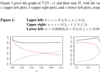
To illustrate (1), I assume Gompertz-Makeham mortality and investigate what happens if two of the parameters are held fixed, while the remaining one takes different values. Figure 1 gives the graph of µ¯−µ0
b ,cx¯and their sumH¯, with the varying parameter being
a(upper left plot),b(upper right plot), andc(lower left plot), respectively.
Figure 1: Upper left:b=c= 0.1,0≤a≤0.1; Upper right:a=c= 0.1,−1≤b≤1; Lower left:a= 0.00002,b= 0.1,0≤c≤0.09
0.00 0.02 0.04 0.06 0.08 0.10
0.0 0.2 0.4 0.6 0.8 1.0 a
−1.0 −0.5 0.0 0.5 1.0
0.0 0.2 0.4 0.6 0.8 1.0 1.2 b
0.00 0.02 0.04 0.06 0.08
0.0 0.2 0.4 0.6 0.8 1.0 c
µ − µ0
b
cx
H=µ − µ0
b +cx
Wrycza: Entropy of the Gompertz-Makeham mortality model
We can see that for an increasingaandb=c = 0.1, the value of µ¯−µ0
b is increasing
while the value ofcx¯is decreasing, resulting in a bathtub-shaped curve forH¯.
Fora=c= 0.1andbincreasing from−1to1, the curve ofcx¯has a reverse sigmoid shape withcx¯≈c·1
c = 1forb=−1,cx¯=c/(a+c) = 0.5forb= 0, andcx¯decreasing
for higher values ofb. µ¯−µ0
b follows a hump-shaped pattern with the maximum atb= 0.
Adding up these two patterns results in a hump-shaped pattern forH¯. However, the maximum here is reachednotatb = 0, but at some negative value ofb, meaning that entropy is highest for a specific pattern of negative senescence.
Fora= 0.00002,b= 0.1(i.e., for values similar to the values encountered in modern human populations) andcincreasing from0to0.09,cx¯is increasing from0to a value close to1in a concave pattern, while ¯µ−µ0
b is decreasing in a convex pattern from a value
close to0.2 to a value close to0. Adding up these curves thus results in a concavely increasing pattern forH¯, starting at a value close to 0.2and approaching1 for higher values ofc.
Relationship (1) allows for a simple calculation ofe†and entropyH¯ in the important case of Gompertz-Makeham mortality. It shows how these quantities relate toe0 = µ1¯ andx¯. As the examples above illustrate, this could provide us with a more systematic understanding of the dynamics between the parametersa,b, andcon the one hand; and the demographically relevant quantitiese0,x¯,e†, andH¯ on the other.
5.
Acknowledgments
Demographic Research: Volume 30, Article 49
References
Demetrius, L. (1974). Demographic Parameters and Natural Selection.Proceedings of the National Academy of Sciences USA71(12): 4645–4547.doi:10.1073/pnas.71.12.4645.
Demetrius, L. (1975). Natural Selection and Age-Structured Populations.Genetics79(3): 535–544.
Demetrius, L. (1976). Measures of Variability in Age-structured Populations. Journal of Theoretical Biology63: 397–404.doi:10.1016/0022-5193(76)90042-4.
Demetrius, L. (1979). Relations Between Demographic Parameters. Demography16(2): 329–338.doi:10.2307/2061146.
Goldman, N. and Lord, G. (1986). A New Look at Entropy and the Lifetable. Demogra-phy23(2): 275–282. doi:10.2307/2061621.
Goldstein, J.R. (2009). Life lived equals live left in stationary populations.Demographic Research20(2): 3–6.doi:10.4054/DemRes.2009.20.2.
Hakkert, R. (1987). Lifetable Transformations and Inequality Measures: Some Notewor-thy Formal Relations.Demography24: 615–622. doi:10.2307/2061396.
Hill, G. (1993). The Entropy of the Survival Curve: An Alternative Measure. Canadian Studies in Population20: 43–57.
Keyfitz, N. (1977a). Applied Mathematical Demography. New York: Wiley.
Keyfitz, N. (1977b). What Difference Would it Make if Cancer Were Eradi-cated? An Examination of the Taeuber Paradox. Demography 14(4): 411–418.
doi:10.2307/2060587.
Leser, C.E.V. (1955). Variations in mortality and life-expectation. Population Studies
9(1): 67–71.doi:10.1080/00324728.1955.10405052.
Mitra, S. (1978). A short note on the Taeuber paradox. Demography15(4): 621–623.
doi:10.2307/2061211.
van Raalte, A.A. and Caswell, H. (2013). Perturbation analysis of indices of lifespan variability.Demography50(5): 1615–1640.doi:10.1080/0032472031000141896.
Vaupel, J.W. (1986). How change in age-speciffc mortality affects life expectancy. Popu-lation Studies40(1): 147–157.doi:10.1080/0032472031000141896.
Vaupel, J.W. (2010). Total incremental change with age equals average lifetime change.
Demographic Research22(36): 1143–1148.doi:10.4054/DemRes.2010.22.36.
Wrycza: Entropy of the Gompertz-Makeham mortality model
Vaupel, J.W. and Canudas Romo, V. (2003). Decomposing Change in Life Expectancy: A Bouquet of Formulas in Honor of Nathan Keyfitz’s 90th Birthday.Demography40(2): 201–2016.doi:10.1353/dem.2003.0018.
Vaupel, J.W., Zhang, Z., and van Raalte, A.A. (2011). Life expectancy and disparity: an international comparison of life table data.BMJ Open1(1). doi:10.1136/bmjopen-2011-000128.
Wagner, P. (2010). Sensitivity of life disparity with respect to changes in mortality rates.
Demographic Research23(3).doi:10.4054/DemRes.2010.23.3.
Wrycza, T.F. and Baudisch, A. (2012). How life-expectancy varies with perturba-tions in age-specic mortality. Demographic Research27(13). doi:10.4054/DemRes. 2012.27.13.
Zhang, Z. and Vaupel, J.W. (2009). The age separating early deaths from late deaths.