DEMOGRAPHIC RESEARCH
A peer-reviewed, open-access journal of population sciences
DEMOGRAPHIC RESEARCH
VOLUME 31, ARTICLE 51, PAGES 1503–1524
PUBLISHED 18 DECEMBER 2014
http://www.demographic-research.org/Volumes/Vol31/51/ DOI: 10.4054/DemRes.2014.31.51
Descriptive Findings
Divergence without decoupling:
Male and female life expectancy usually
co-move
Andrew Noymer
Viola Van
c
2014 Andrew Noymer & Viola Van.
1 Introduction 1504
2 Co-movement and convergence 1505
3 Materials and methods 1506
4 Results and discussion 1517
5 Conclusion 1519
Divergence without decoupling:
Male and female life expectancy usually co-move
Andrew Noymer1
Viola Van2
Abstract
BACKGROUND
Divergence of male and female life expectancy is a well-documented phenomenon. Co-movement is a heretofore-neglected aspect of changes in male and female mortality.
OBJECTIVE
We develop a new framework for life expectancy sex differentials in time series, using co-movement/anti-movement and convergence/divergence.
METHODS
We apply this framework to the Human Mortality Database (HMD), assessing co-move-ment between male and female life expectancy with the nonparametric test of Goodman and Grunfeld (1961).
RESULTS
For every country in the HMD (except three with short spans of data), male and female mortality statistically co-move. This applies even in cases, including ones such as Rus-sia that are well-discussed in the literature, that show extreme divergence between the sexes. The results are reasonably robust to subsetting with a 25-year time-window for all countries.
CONCLUSIONS
Male and female life expectancy co-move even when the life expectancy sex differential increases. The sex divergence in life expectancy needs to be (re-)considered in light of the fact that male and female life expectancy usually co-move, reflecting overall societal factors.
1Department of Population Health and Disease Prevention, University of California, Irvine. 653 E. Peltason
Drive, Irvine CA 92697-3947, USA. E-Mail: [email protected]. The authors would like to thank Leo Good-man for introducing us to and explaining the GoodGood-man-Grunfeld test, and the anonymous referees for useful feedback.
1. Introduction
Women almost always have longer life expectancy than men. This fact is well-ingrained in mortality research, even if the root causes are still debated. While the contribution of behavior (e.g. alcohol or tobacco use) to life expectancy sex differentials is beyond doubt, the counterfactual condition of what mortality differences would look like in the absence of ostensibly changeable behaviors is less clear. A biological basis for some portion of ob-served mortality sex differentials is plausible (Waldron 1983; Garenne and Lafon 1998), although in many settings there is also a social component (see, e.g., Das Gupta 1987; Voland et al. 1997). Even for infant mortality, the role of biology in sex differences is de-bated (Pongou 2013). The long-held interest in mortality sex differentials has generated a large body of literature (e.g., Ciocco 1940a,b; Enterline 1961; Retherford 1975; Preston 1976, 1977; Lopez and Ruzicka 1983; Nathanson 1984; Ram 1993; Vallin 1995; Trovato and Lalu 1996; Kalben 2002; Pampel 2002; Mesl´e 2004; Preston and Wang 2006; Glei and Horiuchi 2007; Luy 2009; Rogers et al. 2010; Oksuzyan et al. 2010; Medalia and Chang 2011; Clark and Peck 2012; Kageyama 2012; Sawyer 2012; Seifarth, McGowan, and Milne 2012; Lindahl-Jacobsen et al. 2013; Thorslund et al. 2013; Oyen et al. 2013), a complete review of which is beyond the current scope.
Our question is whether the forces that shape time series of life expectancy do so in a similar way for males and for females. We do not attempt to explain the existence of the mortality sex differential per se, nor to decompose it among behavioral or biological components. Our interest is in changes of male and female life expectancy, paired at the country level, on a year-to-year basis. This analysis may be indirectly applicable to questions of behavior or biology, but is not designed to test crisp hypotheses about which matters more. Rather, we analyze divergence of male and female life expectancy trajectories using a new analytic framework, that of co-movement, described below.
The divergence of male and female life expectancy has been a topic of much interest, especially in the last 20 years or so (Vallin 1990, 1995; Shkolnikov, Mesl´e, and Vallin 1995; Mesl´e and Vallin 1998; Jasilionis et al. 2011). Adding another dimension, co-movement, uses the same data to reveal different aspects of human mortality, and how these reflect the conditions of the living. This paper examines male:female co-movement of life expectancy in 40 countries around the world. We find that – even when they diverge – males and females almost always statistically co-move.
be-cause male and female life expectancy have become decoupled (or never were coupled), moving their own independent ways with separate drift and noise parameters. This im-plies lack of co-movement: once serial correlation of each series has been dealt with, two independent random walks are not expected to co-move except by chance. Indeed, given the sometimes-enormous sex differences in life expectancy, what is to say – in theory at least – that life expectancy time series need be coupled in the first place? This paper brings an analytic framework and empirical data to bear on these contrasting scenarios.
2. Co-movement and convergence
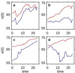
We use the terms “co-movement” and “divergence/convergence” in a specific way. Here-inafter, if two time series are co-moving, then when one goes up, the other one does too, and if one declines, they both decline. Thus, co-movement between two time se-ries means common signs of first differences that are statistically distinguishable from random movement. Statistical co-movement means that the preponderance of moves are in the same direction, not that the two time series need be in lock-step. Only the direc-tion of the movements matters; the magnitudes need not be correlated. The opposite of co-movement is anti-movement. In other words, male and female life expectancies are usually both trending upward, so they have common movements just because of this; cor-recting for serial correlation takes this into account. Convergence has a more intuitive definition: in a specified time window, if two time series are closer together at the end than at the beginning, they are converging. The opposite of convergence is divergence.
Figure 1: Examples of convergence/divergence (left column is convergence; right column is divergence) and co-movement (top row,
co-movement; bottom row, no co-movement). Simulated life expectancy trajectories for men (blue) and women (red). (a) co-movement with convergence; (b) co-movement with divergence; (c) no co-movement, with convergence; (d) no co-movement, with divergence
0
10
20
55
65
75
e(0)
0
10
20
55
65
75
0
10
20
time
55
65
75
e(0)
0
10
20
time
55
65
75
a
b
c
d
3. Materials and methods
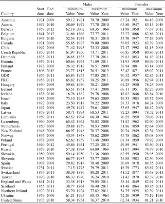
counterex-ample are Russian males, whose life expectancy peaked in 1964, as is well documented (Shkolnikov, Mesl´e, and Vallin 1995; Cockerham 1999; Gavrilova et al. 2008; Billingsley 2011).
Table 1: Descriptive statistics
Males Females
Start End minimum maximum minimum maximum
Country date date Value Year Value Year Value Year Value Year
Australia 1921 2009 59.12 1921 79.70 2009 63.24 1921 84.16 2009
Austria 1947 2010 58.69 1947 77.70 2010 63.80 1947 83.15 2010
Belarus 1959 2012 62.18 2002 69.35 1964 71.98 1959 77.67 2012
Belgium 1841 2012 31.66 1866 77.77 2011 33.27 1866 82.86 2011
Bulgaria 1947 2010 52.54 1947 70.31 2010 55.70 1947 77.26 2009
Canada 1921 2009 55.85 1923 79.00 2009 58.05 1923 83.39 2009
Chile 1992 2008 71.42 1993 75.33 2008 77.47 1992 81.13 2008
Czech Republic 1950 2011 61.97 1950 74.71 2011 66.85 1950 80.86 2011
Denmark 1835 2011 36.65 1835 77.70 2011 39.83 1853 81.83 2011
Estonia 1959 2011 60.64 1994 71.09 2011 71.93 1959 80.99 2011
Finland 1878 2009 26.32 1918 76.51 2009 38.94 1881 83.14 2009
France 1806 2012 23.77 1813 78.51 2012 32.42 1871 85.02 2011
GDR 1956 2011 65.84 1957 77.05 2011 70.52 1957 82.85 2011
FRG 1956 2011 65.82 1957 78.25 2011 70.89 1956 82.94 2011
Hungary 1950 2009 59.85 1950 70.21 2009 64.25 1950 78.23 2009
Ireland 1950 2009 63.51 1951 77.41 2008 66.11 1951 82.23 2009
Iceland 1838 2010 16.76 1882 79.78 2008 18.82 1846 83.84 2010
Israel 1983 2009 73.10 1983 79.63 2009 76.53 1983 83.32 2009
Italy 1872 2009 23.50 1918 79.22 2009 28.33 1918 84.24 2009
Japan 1947 2009 49.78 1947 79.61 2009 53.65 1947 86.42 2009
Latvia 1959 2011 58.71 1994 68.53 2011 72.23 1994 78.52 2011
Lithuania 1959 2011 62.52 1994 68.30 1964 70.55 1959 79.06 2011
Luxemburg 1960 2009 65.42 1964 78.02 2008 71.82 1962 82.90 2009
Netherlands 1850 2009 29.88 1859 78.53 2009 31.86 1859 82.64 2009
New Zealand 1948 2008 66.97 1948 78.37 2008 70.74 1949 82.34 2008
Norway 1846 2009 43.34 1848 78.62 2009 45.78 1862 83.08 2009
Poland 1958 2009 62.62 1959 71.48 2009 68.34 1959 79.92 2009
Portugal 1940 2012 45.86 1941 77.25 2012 49.89 1941 83.50 2011
Russia 1959 2010 57.38 1994 64.89 1964 71.07 1994 74.79 2010
Slovakia 1950 2009 59.14 1950 71.36 2009 62.55 1950 78.95 2009
Slovenia 1983 2009 66.77 1983 75.77 2009 74.88 1983 82.30 2009
Spain 1908 2009 29.82 1918 78.48 2009 30.69 1918 84.55 2009
Sweden 1751 2011 17.15 1773 79.79 2011 18.79 1773 83.67 2011
Switzerland 1876 2011 38.38 1876 80.28 2011 41.52 1877 84.68 2011
Taiwan 1970 2010 66.32 1970 76.24 2010 71.42 1970 82.37 2010
England and Wales 1841 2011 33.38 1918 79.05 2011 38.14 1849 82.94 2011
Scotland 1855 2011 38.77 1864 76.40 2011 41.48 1864 80.85 2011
Northern Ireland 1922 2011 53.70 1924 77.82 2011 54.75 1925 82.39 2011
Ukraine 1959 2009 61.21 1995 68.45 1964 72.20 1959 75.19 1989
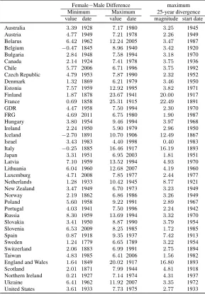
Table 2: Descriptive statistics, female−male difference
Female−Male Difference maximum
Minimum Maximum 25-year divergence
value date value date magnitude start date
Australia 3.39 1928 7.17 1980 3.25 1945
Austria 4.77 1949 7.21 1978 2.26 1949
Belarus 6.42 1962 12.24 2005 3.47 1987
Belgium −0.47 1845 8.96 1940 3.42 1920
Bulgaria 2.84 1948 7.58 1994 3.18 1970
Canada 2.14 1924 7.41 1978 3.75 1936
Chile 5.77 2006 6.71 1996 3.75 1992
Czech Republic 4.79 1953 7.87 1990 2.32 1952
Denmark 1.32 1869 6.21 1979 3.46 1950
Estonia 7.57 1959 12.92 1995 3.82 1971
Finland 1.87 1878 23.67 1941 20.00 1917
France 0.69 1858 25.31 1915 22.49 1891
GDR 4.47 1958 7.50 1994 2.30 1970
FRG 4.69 2011 6.75 1980 1.90 1987
Hungary 3.80 1954 9.46 1994 3.97 1968
Ireland 2.24 1950 5.90 1979 2.96 1950
Iceland −2.70 1891 10.70 1906 12.49 1867
Israel 3.43 1983 4.40 1998 0.40 1983
Italy −0.25 1885 16.46 1917 16.19 1893
Japan 3.31 1951 6.95 2003 1.81 1951
Latvia 7.10 1959 13.52 1994 4.93 1970
Lithuania 6.04 1960 12.68 2007 4.19 1960
Luxemburg 4.71 2008 7.85 1977 2.44 1977
Netherlands 1.28 1933 10.42 1945 8.77 1921
New Zealand 3.47 1949 6.70 1973 3.23 1949
Norway 2.19 1862 6.86 1986 3.26 1949
Poland 5.60 1958 9.22 1991 2.89 1967
Portugal 4.03 1941 7.50 1996 2.24 1942
Russia 8.30 1959 13.69 1994 3.32 1970
Slovakia 3.41 1950 8.87 1990 3.79 1954
Slovenia 6.53 2009 8.25 1985 1.72 1985
Spain 0.87 1918 9.35 1937 7.42 1913
Sweden 1.24 1779 6.65 1789 3.22 1954
Switzerland 2.06 1883 6.99 1991 2.75 1894
Taiwan 4.83 1985 6.41 2006 1.56 1982
England and Wales 1.64 1849 20.02 1917 16.80 1893
Scotland 2.01 1871 7.99 1944 4.81 1918
Northern Ireland 0.21 1927 7.14 1974 4.31 1937
Ukraine 6.41 1962 11.92 2007 3.35 1972
United States 3.61 1933 7.73 1975 2.77 1933
life expectancy. The right two columns of Table 2 give the 25-year window for which the divergence between male and female life expectancy is greatest. For example, for Australia, the period 1945–69 has the greatest 25-year divergence between the sexes in life expectancy: in 1945 the sex difference was 3.68 years (females, 70.35; males, 66.67) and 25 years later the difference was 6.93 (females, 74.70; males, 67.77), for a divergence of 3.25 years. Note, in this example, the end of the 25-year window does not correspond to the single-year maximal sex differential (which was 7.17 years, in 1980), nor does the start correspond to the minimal sex differential (3.39, in 1928). However, there is no 25-year window in the Australian data in which the end-minus-start life expectancy sex differential exceeds 3.25 years.
The countries in the HMD differ in the length of their series. Therefore, we perform a separate analysis, using only the data from the 25-year window for each country. Looking at 25-year subsets is one way to put all the countries on an equal footing, ensuring that differences in statistical significance are not a function of differences in sample size. We choose the 25-year subset in which there is the most divergence to give a conservative estimate of co-movement, since periods of divergence theoretically ought to be when there is the weakest mortality coupling between the sexes. Chile (1992–2008, 17 years) is the only country in the HMD with fewer than 25 years of life expectancy data.
Using the Goodman-Grunfeld (1961) nonparametric test of co-movement between two time series, we analyze signs of first-differences. This approach examines if male and female life expectancy both increase, or both decrease, or move in either permutation of opposite directions, on a year-to-year basis. The Goodman-Grunfeld test is based on the χ2 statistic, but introduces a correction for serial correlation; important, since life expectancy is not a stationary process. The test is also well-suited to small sample sizes (Goodman and Grunfeld 1961).
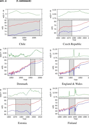
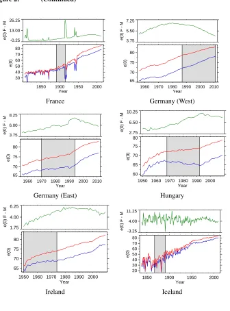
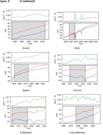
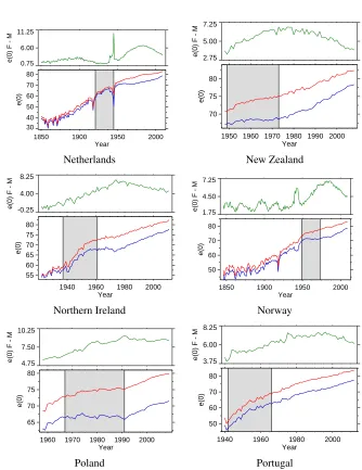
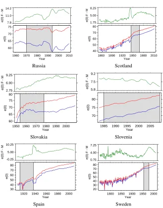
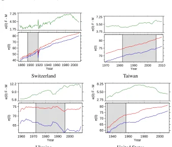
Figure 2: Male and female life expectancy for 6 countries, as labeled. Within each country, the top panel shows the female minus male life expectancy sex differential, and the bottom panel shows male and female life expectancy, with the span of the 25-year window of maxiumum divergence indicated by gray shading
1940 1960 1980 2000 Year 60 65 70 75 80 85 e(0) 2.75 5.50 8.25
e(0) F - M
1950 1960 1970 1980 1990 2000 2010 Year 60 65 70 75 80 85 e(0) 3.75 6.00 8.25
e(0) F - M
Australia Austria
1960 1970 1980 1990 2000 2010 Year 65 70 75 e(0) 5.8 9.5 13.2
e(0) F - M
1850 1900 1950 2000 Year 40 50 60 70 80 e(0) -1.25 4.00 9.25
e(0) F - M
Belarus Belgium
1950 1960 1970 1980 1990 2000 2010 Year 55 60 65 70 75 e(0) 1.75 5.00 8.25
e(0) F - M
1940 1960 1980 2000 Year 55 60 65 70 75 80 85 e(0) 1.75 5.00 8.25
e(0) F - M
Figure 2: (Continued)
1995 2000 2005
Year 72 74 76 78 80 82 e(0) 5 6 7
e(0) F - M
1950 1960 1970 1980 1990 2000 2010 Year 65 70 75 80 e(0) 3.75 6.00 8.25
e(0) F - M
Chile Czech Republic
1850 1900 1950 2000
Year 40 50 60 70 80 e(0) 0.75 4.00 7.25
e(0) F - M
1850 1900 1950 2000
Year 40 50 60 70 80 e(0) 0.75 11.00 21.25
e(0) F - M
Denmark England & Wales
1960 1970 1980 1990 2000 2010
Year 60 65 70 75 80 e(0) 6.8 10.0 13.2
e(0) F - M
1880 1900 1920 1940 1960 1980 2000 Year 30 40 50 60 70 80 e(0) 0.75 12.50 24.25
e(0) F - M
Figure 2: (Continued)
1850 1900 1950 2000
Year 30 40 50 60 70 80 e(0) -0.25 13.00 26.25
e(0) F - M
1960 1970 1980 1990 2000 2010
Year 65 70 75 80 e(0) 3.75 5.50 7.25
e(0) F - M
France Germany (West)
1960 1970 1980 1990 2000 2010
Year 65 70 75 80 e(0) 3.75 6.00 8.25
e(0) F - M
1950 1960 1970 1980 1990 2000 Year 60 65 70 75 80 e(0) 2.75 6.50 10.25
e(0) F - M
Germany (East) Hungary
1950 1960 1970 1980 1990 2000 Year 65 70 75 80 e(0) 1.75 4.00 6.25
e(0) F - M
1850 1900 1950 2000
Year 20 30 40 50 60 70 80 e(0) -3.25 4.00 11.25
e(0) F - M
Figure 2: (Continued)
1985 1990 1995 2000 2005
Year 74 76 78 80 82 84 e(0) 2.75 4.00 5.25
e(0) F - M
1880 1900 1920 1940 1960 1980 2000 Year 30 40 50 60 70 80 e(0) -1.25 8.00 17.25
e(0) F - M
Israel Italy
1950 1960 1970 1980 1990 2000 Year 50 60 70 80 e(0) 2.75 5.00 7.25
e(0) F - M
1960 1970 1980 1990 2000 2010
Year 60 65 70 75 80 e(0) 6.8 10.5 14.2
e(0) F - M
Japan Latvia
1960 1970 1980 1990 2000 2010
Year 65 70 75 80 e(0) 5.8 9.5 13.2
e(0) F - M
1960 1970 1980 1990 2000
Year 65 70 75 80 e(0) 3.75 6.00 8.25
e(0) F - M
Figure 2: (Continued)
1850 1900 1950 2000
Year 30 40 50 60 70 80 e(0) 0.75 6.00 11.25
e(0) F - M
1950 1960 1970 1980 1990 2000 Year 70 75 80 e(0) 2.75 5.00 7.25
e(0) F - M
Netherlands New Zealand
1940 1960 1980 2000
Year 55 60 65 70 75 80 e(0) -0.25 4.00 8.25
e(0) F - M
1850 1900 1950 2000
Year 50 60 70 80 e(0) 1.75 4.50 7.25
e(0) F - M
Northern Ireland Norway
1960 1970 1980 1990 2000
Year 65 70 75 80 e(0) 4.75 7.50 10.25
e(0) F - M
1940 1960 1980 2000
Year 50 60 70 80 e(0) 3.75 6.00 8.25
e(0) F - M
Figure 2: (Continued)
1960 1970 1980 1990 2000 2010
Year 60 65 70 75 e(0) 7.8 11.0 14.2
e(0) F - M
1860 1890 1920 1950 1980 2010
Year 40 50 60 70 80 e(0) 1.75 5.00 8.25
e(0) F - M
Russia Scotland
1950 1960 1970 1980 1990 2000 Year 60 65 70 75 80 e(0) 2.75 6.00 9.25
e(0) F - M
1985 1990 1995 2000 2005 Year 70 75 80 e(0) 5.8 7.5 9.2
e(0) F - M
Slovakia Slovenia
1920 1940 1960 1980 2000
Year 30 40 50 60 70 80 e(0) -0.25 5.00 10.25
e(0) F - M
1800 1850 1900 1950 2000
Year 20 30 40 50 60 70 80 e(0) 0.75 4.00 7.25
e(0) F - M
Figure 2: (Continued)
1880 1900 1920 1940 1960 1980 2000 Year
40 50 60 70 80
e(0)
1.75 4.50 7.25
e(0) F - M
1970 1980 1990 2000 2010
Year 70
75 80
e(0)
3.75 5.50 7.25
e(0) F - M
Switzerland Taiwan
1960 1970 1980 1990 2000
Year 65
70 75
e(0)
5.8 9.0 12.2
e(0) F - M
1940 1960 1980 2000
Year 60
65 70 75 80
e(0)
2.75 5.50 8.25
e(0) F - M
4. Results and discussion
Table 3 presents the results of the Goodman-Grunfeld tests. When using the entire time series for each country, only three countries do not have significant co-movement of life expectancy between the sexes. These are Chile, which has only 17 years of data, Lux-embourg, which has ample data, and Slovenia (only 27 years of data). The negative test statistic for Luxembourg (Table 3) is nowhere near large enough to indicate statistically-significant anti-movement if the opposite one-sidedp-value were to be calculated; it is simply non-significant. All the other G-G test statistics reject the null hypothesis of no co-movement at the 5% level. Clearly, the overall picture is that male and female life expectancies co-move.
Table 3 also gives the proportion of the co-movements which are congruent. This may be thought of like an effect size, as opposed to a test of statistical significance. For most of the populations, the proportion of congruent co-movements is high – for example of the 37 statistically-significant countries, 22 have an 85% or greater proportion of congruent co-movements. On the other hand, as the most extreme example of a modest effect size, consider New Zealand. With a test statistic of2.439, it is amply significant (p= 0.0074), while the co-movements are congruent73.3%of the time. This is clearly still a majority of congruent co-movements but shows that effect size does not always follow thep-value. Of the 37 statistically-significant countries, there are 10 with less than 80%congruent co-movements (80%could nonetheless still be regarded as a somewhat strict criterion). Luxembourg shows only51% congruent co-movements, but of course it was far from significant in the G-G test.
Table 3: Goodman-Grunfeld test statistics andp-values
Entire Series 25-year Window
G-G test one-sided proportion G-G test one-sided proportion
statistic p-value congruent statistic p-value congruent
Australia 5.610 <.00005 0.852 3.468 0.0003 0.958
Austria 3.386 0.0004 0.873 2.239 0.0126 0.833
Belarus 3.979 <.00005 0.792 2.514 0.0060 0.792
Belgium 9.895 <.00005 0.892 2.820 0.0024 0.833
Bulgaria 5.627 <.00005 0.873 2.097 0.0180 0.750
Canada 5.988 <.00005 0.909 1.418 0.0781 0.792
Chile 1.047 0.1476 0.812 1.047 0.1476 0.812
Czech Republic 5.552 <.00005 0.918 2.576 0.0050 0.833
Denmark 8.779 <.00005 0.852 1.073 0.1416 0.708
Estonia 3.175 0.0007 0.750 1.593 0.0556 0.708
Finland 7.796 <.00005 0.863 2.973 0.0015 0.875
France 11.574 <.00005 0.917 4.089 <.00005 0.958
GDR 4.926 <.00005 0.909 3.229 0.0006 0.917
FRG 4.039 <.00005 0.891 — — 0.875
Hungary 3.901 <.00005 0.780 2.465 0.0069 0.750
Ireland 2.711 0.0034 0.763 2.723 0.0032 0.833
Iceland 5.216 <.00005 0.715 3.749 0.0001 0.917
Israel 1.930 0.0268 0.846 1.784 0.0372 0.833
Italy 9.243 <.00005 0.920 3.172 0.0008 0.958
Japan 5.523 <.00005 0.935 3.132 0.0009 1.0
Latvia 3.029 0.0012 0.731 1.496 0.0673 0.708
Lithuania 3.361 0.0004 0.731 1.614 0.0532 0.625
Luxemburg −0.088 0.5351 0.510 −0.429 0.6660 0.542
Netherlands 8.682 <.00005 0.862 3.702 0.0001 0.917
New Zealand 2.439 0.0074 0.733 2.026 0.0214 0.792
Norway 7.890 <.00005 0.828 1.753 0.0398 0.667
Poland 4.548 <.00005 0.863 2.328 0.0100 0.750
Portugal 5.984 <.00005 0.903 4.349 <.00005 1.0
Russia 4.708 <.00005 0.843 2.781 0.0027 0.833
Slovakia 3.317 0.0005 0.780 2.709 0.0034 0.833
Slovenia 1.341 0.0899 0.846 1.224 0.1105 0.833
Spain 7.032 <.00005 0.891 3.215 0.0007 0.917
Sweden 12.997 <.00005 0.912 1.512 0.0653 0.708
Switzerland 7.100 <.00005 0.859 4.322 <.00005 1.0
Taiwan 2.854 0.0022 0.875 2.260 0.0119 0.833
England and Wales 11.073 <.00005 0.941 3.400 0.0003 0.875
Scotland 8.090 <.00005 0.846 3.373 0.0004 0.917
Northern Ireland 4.237 <.00005 0.787 2.184 0.0145 0.833
Ukraine 4.163 <.00005 0.820 1.671 0.0473 0.750
United States 6.760 <.00005 0.948 3.790 0.0001 1.0
it is not a separate test, since the country only has 14 years of data; in Slovenia (27 years of data total), the 25-year window is nearly the same test as the overall series; and in Lux-embourg, the 25-year window has a similar character as the overall 50-year data set. The six countries for which there is a lack of significant co-movement at the 5% level for the 25-year window, despite significant co-movement in the entire data series, are Canada, Denmark, Estonia, Latvia, Lithuania, and Sweden. During their periods of maximum di-vergence, these countries behave like panel (d) of Figure 1, with divergence accompanied by decoupling of male and female life expectancy (viz., lack of co-movement). However, among the six countries, only Denmark would fail to reject the null at the 10% signifi-cance level. There are 24 first-difference values in each of these windows – a sample size that is unusually low, even for country-level studies. For the 25-year window, no G-G test may be performed for West Germany (FRG in Table 3); this stems from the monotonic increase of male life expectancy in this time period.
This study has several limitations. The HMD is not a representative sample of the global population; it only includes countries whose data meet its quality control standards. Caution is therefore warranted when extrapolating from the HMD to the world as a whole. As noted, the HMD data series are not of equal length; this makes country-by-country comparisons of statistical significance problematic. The extreme case, Chile, has a data set with 16 first-differences. We have tried to address this in two ways. First, we use a Neyman-Pearson (not Fisherian) statistical framework (Lehmann 1993 discusses the distinction): results are considered as significant/not-significant without bias toward the large test statistics (i.e., smallp-values) that come out of the longer time series. Second, we have done a set of comparisons using the same window size (25 years, maximum divergence) for all countries. The choice of maximum divergence is to make the test conservative: intuitively, one would expect divergence to favor non-co-movement, as in panel (d) of Figure 1. However, the choice of 25 years is arbitrary.
5. Conclusion
Preston and colleagues (1972) commented, “mortality conditions mirror those in the gen-eral society”. This makes sex differences all the more interesting, since mortality sex differentials change frequently. Extreme sex differences are associated with wartime. However, even in peacetime there are a number of large sex differentials, most notably Russia in 1994, when female life expectancy exceeded that of males by 13.7 years. All peacetime sex differences≥11 years occur in former Soviet countries, in 1994 or later.
divergence – and, in some cases, convergence, as women adopt previously “male” be-haviors such as tobacco use (e.g. Preston and Wang 2006). This raises the question, are males and femalesseparatebarometers of conditions in the general society?
This study gives a nuanced answer to that question. When it comes to life expectancy, co-movement is the norm – all but three of the 40 HMD countries show significant co-movement when evaluated on their entire data series. Moreover, the preponderance (31 countries) still show significant co-movement when evaluated on the 25-year most-divergent subset. This is surprising given the extreme nature of these subsets: 25-years is a very short time window, stacking the deck in favor of type II errors; choosing the most-divergent period intuitively would seem to be a set-up forlackof co-movement.
We interpret these co-movement findings as follows. Severe or lenient mortality con-ditions act in the same direction on both sexes. Thus, changes in the overall mortal-ity environment cause male and female life expectancy to co-move. Remarkably, even when male and female life expectancy trends are diverging, this usually applies. Life expectancy sex divergence has much to teach us, and reflects important aspects of soci-ety. However, it does not reveal much about “conditions . . . in the general society”, but, rather, about sex-specific risk behavior (alcohol abuse, tobacco use, violence) or labor force participation (Pampel and Zimmer 1989). On the other hand, the overall trend of mortality does indeed reflect conditions in the general society, but – as demonstrated by the analysis herein – these tend to act similarly on both sexes. As Vallin (1990) noted, “Time trends . . . reflect general health progress, which results in a gain in life expectancy for both sexes, but more so for women, among whom adverse health behaviours have traditionally been less common.”
References
Billingsley, S. (2011). Exploring the conditions for a mortality crisis: Bringing context back into the debate. Population, Space and Place17(3): 267–289. doi:10.1002/psp. 660.
Ciocco, A. (1940a). Sex differences in morbidity and mortality. Quarterly Review of Biology15(1): 59–73. doi:10.1086/394601.
Ciocco, A. (1940b). Sex differences in morbidity and mortality (concluded). Quarterly Review of Biology15(2): 192–210.doi:10.1086/394601.
Clark, R. and Peck, B.M. (2012). Examining the gender gap in life expectancy: A cross-national analysis, 1980–2005. Social Science Quarterly93(3): 820–837. doi:10.1111/ j.1540-6237.2012.00881.x.
Cockerham, W.C. (1999).Health and social change in Russia and Eastern Europe. New York: Routledge.
Das Gupta, M. (1987). Selective discrimination against female children in rural Punjab, India. Population and Development Review13(1): 77–100.doi:10.2307/1972121.
Enterline, P.E. (1961). Causes of death responsible for recent increases in sex mortality differentials in the United States. Milbank Memorial Fund Quarterly39(2): 312–328.
doi:10.2307/3348603.
Garenne, M. and Lafon, M. (1998). Sexist diseases.Perspectives in Biology and Medicine 41(2): 176–189.
Gavrilova, N.S., Semyonova, V.G., Dubrovina, E., Evdokushkina, G.N., Ivanova, A.E., and Gavrilov, L.A. (2008). Russian mortality crisis and the quality of vital statistics. Population Research and Policy Review 27(5): 551–574. doi:10.1007/s11113-008-9085-6.
Glei, D.A. and Horiuchi, S. (2007). The narrowing sex differential in life expectancy in high-income populations: Effects of differences in the age pattern of mortality. Popu-lation Studies61(2): 141–159.doi:10.1080/00324720701331433.
Goodman, L.A. and Grunfeld, Y. (1961). Some nonparametric tests for comovements between time series. Journal of the American Statistical Association56(293): 11–26.
doi:10.1080/01621459.1961.10482086.
Human Mortality Database (2014). Human mortality database. http://www.mortality. org/, Accessed 15 March 2014.
doi:10.1007/s10680-011-9243-0.
Kageyama, J. (2012). Happiness and sex difference in life expectancy. Journal of Hap-piness Studies13(5): 947–967. doi:10.1007/s10902-011-9301-7.
Kalben, B.B. (2002). Why men die younger: Causes of mortality differences by sex. Schaumburg, IL: Society of Actuaries.
Lehmann, E.L. (1993). The Fisher, Neyman-Pearson theories of testing hypotheses: One theory or two? Journal of the American Statistical Association88(424): 1242–1249.
doi:10.1080/01621459.1993.10476404.
Lindahl-Jacobsen, R., Hanson, H.A., Oksuzyan, A., Mineau, G.P., Christensen, K., and Smith, K.R. (2013). The male-female health-survival paradox and sex differences in cohort life expectancy in Utah, Denmark, and Sweden 1850–1910.Annals of Epidemi-ology23(4): 161–166.doi:10.1016/j.annepidem.2013.02.001.
Lopez, A.D., Caselli, G., and Valkonen, T. (eds.) (1995). Adult mortality in developed countries: From description to explanation. Oxford: Clarendon Press/Oxford Univer-sity Press.
Lopez, A.D. and Ruzicka, L.T. (eds.) (1983). Sex differentials in mortality: Trends, determinants and consequences. Canberra: Australian National University.
Luy, M. (2009). Unnatural deaths among nuns and monks: Is there a biological force behind male external cause mortality? Journal of Biosocial Science41(6): 831–844.
doi:10.1017/S0021932009990216.
Medalia, C. and Chang, V.W. (2011). Gender equality, development, and cross-national sex gaps in life expectancy. International Journal of Comparative Sociology52(5): 371–389.doi:10.1177/0020715211426177.
Mesl´e, F. (2004). Ecart d’esp´erance de vie entre les sexes: Les raisons du recul de´ l’avantage f´eminin. Revue d’ ´Epid´emiologie et de Sant´e Publique52(4): 333–352.
doi:10.1016/S0398-7620(04)99063-3.
Mesl´e, F. and Vallin, J. (1998). ´Evolution et variations g´eographiques de la surmortalit´e masculine: Du paradox franc¸ais `a la logique russe. Population 53(6): 1079–1102.
doi:10.2307/1534966.
Nathanson, C.A. (1984). Sex differences in mortality. Annual Review of Sociology10: 191–213.doi:10.1146/annurev.so.10.080184.001203.
Oksuzyan, A., Crimmins, E., Saito, Y., O’Rand, A., Vaupel, J.W., and Christensen, K. (2010). Cross-national comparison of sex differences in health and mortality in Denmark, Japan and the US. European Journal of Epidemiology 25(7): 471–480.
Oyen, H., Nusselder, W., Jagger, C., Kolip, P., Cambois, E., and Robine, J.M. (2013). Gender differences in healthy life years within the EU: An exploration of the ‘health-survival’ paradox.International Journal of Public Health58(1): 143–155.
doi:10.1007/s00038-012-0361-1.
Pampel, F.C. (2002). Cigarette use and the narrowing sex differential in mortality. Popu-lation and Development Review28(1): 77–104.doi:10.1111/j.1728-4457.2002.00077. x.
Pampel, F.C. and Zimmer, C. (1989). Female labour force activity and the sex differential in mortality: Comparisons across developed nations, 1950–1980.European Journal of Population5(3): 281–304.doi:10.1007/BF01796820.
Pongou, R. (2013). Why is infant mortality higher in boys than in girls? A new hypoth-esis based on preconception environment and evidence from a large sample of twins. Demography50(2): 421–444. doi:10.1007/s13524-012-0161-5.
Preston, S.H. (1976). Mortality patterns in national populations: With special reference to recorded causes of death. New York: Academic Press.
Preston, S.H. (1977). Mortality tends. Annual Review of Sociology 3: 163–178.
doi:10.1146/annurev.so.03.080177.001115.
Preston, S.H., Keyfitz, N., and Schoen, R. (1972). Causes of death: Life tables for national populations. New York: Seminar Press.
Preston, S.H. and Wang, H. (2006). Sex mortality differentials in the United States: The role of cohort smoking patterns.Demography43(4): 631–646.doi:10.1353/dem.2006. 0037.
Ram, B. (1993). Sex differences in mortality as a social indicator. Social Indicators Research29(1): 83–108.doi:10.1007/BF01136198.
Retherford, R.D. (1975).The changing sex differential in mortality. Westport, Connecti-cut: Greenwood Press.
Rogers, R.G., Everett, B.G., Onge, J.M.S., and Krueger, P.M. (2010). Social, behavioral, and biological factors, and sex differences in mortality. Demography47(3): 555–578.
doi:10.1353/dem.0.0119.
Sawyer, C.C. (2012). Child mortality estimation: Estimating sex differences in childhood mortality since the 1970s.PLoS Medicine9(8): e1001287. doi:10.1371/journal.pmed.
1001287.
Shkolnikov, V., Mesl´e, F., and Vallin, J. (1995). La crise sanitaire en Russie. I. tendances r´ecentes de l’esp´erance de vie et des causes de d´ec`es de 1970 `a 1993. Population 50(4/5): 907–943.doi:10.2307/1534310.
Thorslund, M., Wastesson, J.W., Agahi, N., Lagergren, M., and Parker, M.G. (2013). The rise and fall of women’s advantage: A comparison of national trends in life expectancy at age 65 years. European Journal of Ageing10(4): 271–277. doi:10.1007/s10433-013-0274-8.
Trovato, F. and Lalu, N.M. (1996). Narrowing sex differentials in life expectancy in the industrialized world: Early 1970’s to early 1990’s.Social Biology43(1–2): 21–37.
Vallin, J. (1990). Quand les variations g´eographiques de la surmortalit´e masculine con-tredisent son ´evolution dans le temps. Espace, Populations, Soci´et´es8(3): 467–478.
doi:10.3406/espos.1990.1426.
Vallin, J. (1995). Can sex differentials in mortality be explained by socio-economic mor-tality differentials? In: Lopez, Caselli, and Valkonen (1995), 179–200.
Vallin, J. and Mesl´e, F. (2001).Tables de mortalit´e franc¸aises pour les XIXeet XXesi`ecles et projections pour le XXIesi`ecle. Paris: Institut national d’´etudes d´emographiques.
Voland, E., Dunbar, R.I.M., Engel, C., and Stephan, P. (1997). Population increase and sex-biased parental investment in humans: Evidence from 18th- and 19th-century Ger-many.Current Anthropology38(1): 129–135.doi:10.1086/204593.