Predator-prey interactions with harvesting of predator with prey in refuge

*

Corresponding author Received September 20, 2012

1

Available online at http://scik.org

Commun. Math. Biol. Neurosci. 2013, 2013:1

PREDATOR-PREY INTERACTIONS WITH HARVESTING OF

PREDATOR WITH PREY IN REFUGE

S. A. WUHAIB*, Y. ABU HASAN

School of Mathematical Sciences, Universiti Sains Malaysia, Penang, Malaysia

Abstract: In this paper,we study predator prey interactions where the predator is exposed to the risk of disease and harvesting while the prey has the ability to use a refuge. We consider two models: the ability of prey to use a constant refuge and the ability to use random refuge. We found bounded, non-periodic solutions and the equilibrium points for both models. We then show the role of the refuges in the stability of the systems. The equilibrium was stable locally, but not globally, and we found some basin to these equilibrium points. Numerical simulations show several types of oscillations that occur due to the kinds of refuges and prey's ability to use these refuges. For both models, there exist an invariant region; the invariant region in the constant refuge is better than the invariant region in random refuge because it ensures the continuity of all populations and sustainability of the harvested species and controlling the disease without it becoming endemic. Finally the low density prey in refuges makes a limit cycle around the equilibrium in refuges whiles the small density is stable.

Keywords: Constant Refuge; Random Refuge; Basin of attraction; Limit cycle.

2000 AMS Subject Classification: 92B05

1. Introduction

Prey-predator models are of great interest to researchers in mathematics and ecology

because they deal with environmental problems such as community’s morbidity and

how to control it, optimal harvest policy to sustain a community, and others. In the

phenomena. However, in the life sciences a model only describes a particular situation.

Simple models such as the Lotka-Volterra are not able to tell us what is going on in

the majority of cases. One of the reasons is due to the complexity of the biological

ecosystem. Hence the needs for a variety of models to describe nature .

Theoretical and numerical studies of these models are able to give us an

understanding of the interactions that is taking place. A particular class of models

considers the existence of a disease in the predator or prey. Several models were

constructed to study particular cases. To ensure the existence of the species involved,

one of the steps taken is to harvest the infected species. Due to the need to survive, the

prey has developed strategies to avoid the predator, one of them the use of refuge.

In this paper, we consider the case where the infected predator is harvested, while the

prey has a refuge. Several related theoretical studies have been conducted.

Amongst them are studies on the disease spread among the prey and the epidemic

among predators with action incidence [18], the role of transmissible disease in the

Holling Tanner predator prey model [9], the analysis of prey predator model with

disease in the prey [19], anothers study the disease in Lotka Volterra, [7]study the

dynamics of a fisher resource system in an aquatic environment in two zones harvest

in reserve area,[16] study the harvesting of infected prey,[2]show the stability analysis

of harvesting,[6] Study the stability of harvested when the disease affects the predator

by using the reproduction number, While some researchers took their studies using the

refuge by the prey and the types of those refuges where used ,[4] idea refuge disk with

response function type II functional response incorporation a constant prey refuge[3]

studied the idea of using prey refuge random,[1,4]Some studies took the form of a

special like the refuges effect on the stability of the models studied in [14,11, 10],[17,

8] the refuge protect a constant number of prey lead to a stable and stronger

stabile ,[13 , 6 ,8] investigated that the a destabilizing effect through the occurrence of

a stable limit cycle. Analysis [15] refers to the low density of prey at the refuge gives

a limit cycle,[15] investigated the rate at which prey moves to refuge is proportional

kinds of refuge (constant and proportional) and investigated the role of these in

different classes of functional responses.

The model is introduced after this section, followed by analysis on nature and

properties of the solutions. Numerical simulations were performed to verify the

theoretical discussions and to investigate further properties.

2. Mathematical model

The model is written as:





1

2

(1 ) (1 )

(1 )

(1 )

x rx x ax m y z

y bx m y yz q y

z bx m z yz q z

 

    

 

   



    



(1)

where x, y, z are the prey, infected predator and susceptible predator respectively; r is the growth rate of prey; a ,b the capture rate (ab),is the contact rate between the susceptible and infected predator; q q₁, ₂ are the harvest rates of the infected and susceptible predator respectively,mis a constant (which describes the ability of the prey to use constant refuge) . We assume that the less effective predator shall be easier to harvest, soq₁ q₂; we also assume infected predator not become susceptible again and finally the disease does not affect the ability of the infected predator attacking prey .

2.1 Nature of solutions

Theorem 1.The solution of system (1) is bounded.

Proof .

Let the function w x y z( , , )x t( )y t( )z t( ) and take the positive number

2

0  q

Then w t

 

uwrx(1 x) x



a b x



(1m)



y z

 

q₁

 

y q₂



z

 

2 2 1 2

2 2

r r r

r x

r

t uw x

r w

r

  

 _{     }  _{  }   _ _{ } _{ } _ _{ }

     

 

2

1 Let

2

r

v r





 _{ }

 

 

 

 

w t uw t v













0

0 , , 1 ut ut , , |

t

v

w x y z e e x y z

u

 



   

Theorem 2.The system (1) has no periodic solution

Proof.

To show there is no periodic orbit to this system, we use Dulac’s criterion and first

consider the xy-plane,

Leth x y₁

 

,  rx rx2ax(1m y) , h₂



x y,



bx(1m y) q y₁

 

x y,



h H1





h H2



r

x y y

 

 

    

It’s clear that is no change in sign, therefore this system cannot have any periodic

solution in the xy- plane.

LetH x z( , ) 1

xz

 , where H x z( , )in the positive quadrant of the xz- plane

Leth x z₃

 

,  rx rx2ax(1m z) , h x z₄

 

, bx(1m z q z)  ₂

 

x z,



h H3





h H4



r

x z z

 

 

    

There is no change in sign; therefore there is no periodic solution in xz- plane.

Hence the system has no periodic solution.

2.2 Equilibrium

Letting



x  y z 0



we get the equilibriums (non trivial):

 

i A predator free-equilibriumP_c1(1, 0, 0) in the absent of the predator, the prey

grows and tends to its carrying capacity.

the system,where 2 2

2 2

(1 ) ,

(1 ) (1 )

q r x

x z

b m a m



 

 

( )iii The disease becomes epidemic i.e. all predators become infected, the

equilibrium in this caseP x y_c3( ,_{3 3}, 0), where 1 3

3 3

(1 ) ,

(1 ) (1 )

r x

q

x y

b m a m



 

 

( )iv The positive equilibrium Pc (x y z, , )

   

where all population coexists and

survives, from the second and third equations of system (1) we get

1 2 1 2 (1 ) (1 )

bx m z q

bx m y q

q q y z             

Then



1 2



2 1

(1 ) (1 )

1 a (1 ) , bx m q , q bx m

x m q q y z

r  

 

_{   }  _   _  

With conditions



1 2



1 2

1 r m and 1 q m 1 q

a q q bx bx

         

2.2. Equilibrium

Letting



x  y z 0



we get the equilibriums (non trivial):

 

i A predator free-equilibriumP_c1(1, 0, 0) in the absent of the predator, the prey

grows and tends to its carrying capacity.

( )ii A disease free equilibriumP_c2( , 0,x₂ z₂), in this case the disease disappears

from the system,where 2 2

2 2

(1 ) ,

(1 ) (1 )

q r x

x z

b m a m



 

 

( )iii The disease becomes epidemic i.e. all predators become infected, the

equilibrium in this caseP x y_c3( ,_{3 3}, 0), where 1 3

3 3

(1 ) ,

(1 ) (1 )

r x

q

x y

b m a m



 

 

( )iv The positive equilibrium Pc (x y z, , )

   

where all population coexists and

1 2 1 2 (1 ) (1 )

bx m z q

bx m y q

q q y z             

Then





2 1

1 2

(1 ) (1 )

1 a (1 ) , bx m q , q bx m

x m q q y z

r  

 

_{   }  _   _  

With conditions



1 2



1 2

1 r m and 1 q m 1 q

a q q bx bx

         

2.3. Stability

The Jacobian matrix of system (1) is given by:

1

2

2 (1 )( ) (1 ) (1 )

(1 ) (1 )

(1 ) (1 )

c

r rx a m y z ax m ax m

J b m y bx m z q y

b m z z bx m y q

                _     _         

First we study system (1) as a sub system (without disease); the system become

2

(1 ) (1 )

(1 )

x rx x ax m z

z bx m z q z

   



   

 (1-a)

The equilibrium (non trivial) areE_c(1, 0),E x z_c( ,_{2 2})), where

2 2

2 2

1 and

(1 ) 1

q r x

x z

b m a m



 

 _{  }

   

The eigenvalues near the first equilibrium are rand b(1m)q₂ .

This is stable when 2

1 q

m

b

  and unstable otherwise.

Let R0is denote the basic reproduction number of the susceptible predator, where

0 2 (1 ) b m R q 

 and if R₀ 1the susceptible predator survive, but in this caseR₀ 1;

therefore the second eigenvalues is negative then this equilibrium is stable. This

stability can become unstable when we change one or all the parameters



q m b₂, ,



_.

therefore it is stable without any condition. We cannot find the Lyapunov function at

this point to proof a global asymptotically stable in 2

R_, In the following theorem we

show the basin of attraction ofE x z_c( ,_{2 2}).

Theorem 3. Assume that the equilibriumE x z_c( ,_{2 2}) is locally stable, the basin of

attraction of this equilibrium is denoted byB E x z( _c( ,_{2 2}) where





2

2 2 2 2 2 2

( _c( , ) {( , ) : , , with }

B E x z  x z R xx zz x zz x

Proof.

Let V x z₁( , )be a function where

1 2 2 2 2

2 2

( , ) log x log z

V x z x x x z z z

x z

   

_   _{ }   _

    ,then



 

2









2 1

2 2

(1 ) 0

r x x a b m

dV

z z

dt      xx  

The eigenvalues near P x₂( , 0,₂ z₂)are





2 2

2 2 2

2 4 1

2 2

r x q r x

rx  

 _

and q₂z₂q₁

It is stability when



1 22



(1 )

1 r x m

a q q

 

 



When all predators become infected the subsystem become as

1

(1 ) (1 )

(1 )

x rx x ax m y

y bx m y q y

   



   

 (1-b)

The equilibriums (non trivial) are E_c(1, 0),E x yˆ_c( ,_{3 3})where,

3 1

3 3

(1 ) ,

(1 ) (1 )

r x

q

x y

b m a m



 

 

And the eigenvalues near E_c(1, 0)are r andb(1m)q1, this is stable when

1

1 q

m

b

  and unstable otherwise.

Let R₁is denotes the basic reproduction number of the infected predator, where

1 1 (1 ) b m R q 

therefore the second eigenvalues is negative then this equilibrium is stable. This

stability can transform to unstable when we decrease one or all parameters



q m b₁, ,



.

The trace of Jacobian matrix near the equilibriumE x yˆ ( , )_{c 3 3} is rx₃ (negative)

therefore it is stable without any condition. We can find the basin of attraction to this

point as in the following theorem.

Theorem 4. Assume that the equilibriumE x yˆ ( , )_{c 3 3} is locally stable, the basin of

attraction of this equilibrium is denoted byB E x y



ˆ ( , )_{c 3 3}



where

2

3 3 3 3

( _c( , ) {( , ) : , }

B E x y  x z R_ xx yy

Proof.

The proof is same in theorem (3).

The equilibriumP x y_c3( ,_{3 3}, 0) is stable with condition



1 32



(1 )

1 r x

m

a q q

 

 

 .

The stability near the equilibriumP_c(x y z, , )is given by the equation

3 2

0

A B C

      Where







2 2



2

0 , (1 ) , 0

Arx  B ax b m yz  y z  C r x y z  







2



(1 ) 0

AB C rx ax b  m yz 

From Routh- Hurwitz stability criterion it is stable.

Theorem 5. Assume that the equilibriumP_c(x y z, , ) is locally stable, the basin of

attraction of this equilibrium is denoted byB P x y z



_c( , , )



where

3

( _c ( , , ) ) {( , , ) : , , }

B P x y z     x y z R_ xx y y z z

Proof.

The proof is similar to proof of theorem (3).

3. The random refuge model





1

2

(1 ) ( )

( )

( )

x rx x a x m y z

y b x m y yz q y

z b x m z yz q z

 

    



 _{   }



    



(2)

3.1 Nature of solution.

Theorem 6 .The solution of system (2) is bounded.

Proof.

Let the function w x y z( , , )x t( )y t( )z t( ) and take the positive number

2

0  q

Then w

 

t uwrx(1 x) x



a b



(xm)



yz

 

 q₁

 

y q₂



z

 

2 2 1 2

2 2

r r r

r x

r

t uw x

r w

r

  

 _{     }  _{  }   _ _{ } _{ } _ _{ }

     

 

 

2

1 Let

2

r

v r





 _{ }

 

 

 

 

w t uw t v













0

0 , , 1 ut ut , , |

t

v

w x y z e e x y z

u

 



   

Theorem 7.The system (2) has no periodic solution

Proof.

To show there is no periodic orbit to this system, we use Dulac’s criterion and first

consider the xy-plane,

Leth x y₁

 

,  rx rx2a x m y(  ) ,h₂



x y,



b x( m y) q y₁ ,and





1

,

H x y xy

 , where H x z( , )in the positive quadrant of the xy- plane, then

 



1





2



2

, h H h H r am

x y

x y y x

 

 

     

It’s clear that is no change in sign, therefore this system cannot have any periodic

LetH x z( , ) 1

xz

 , where H x z( , )in the positive quadrant of the xz- plane, and

 

2

3 , ( )

h x z  rx rx a x m z , h x z₄

 

, b x m z q z(  )  ₂

 



3





4



2

, h H h H r am

x z

x z z x

 

 

     

There is no change in sign; therefore there is no periodic solution in xz- plane.

Hence the system has no periodic solution.

3.2 Equilibrium

Again by letting



x  y z 0



we get the equilibriums (non trivial):

 

i A predator free-equilibriumP_r1(1, 0, 0), in the absent of the predator, the prey

grows and tends to its carrying capacity.

( )ii A disease free equilibriumP_r2( , 0,x₂ z₂), in this case the disease disappears from

the systemand 2 2 2

2 2

2

(1 ) ,

( )

q rx x

x m z

b a x m



  



( )iii The disease become an epidemic i.e. all predators become infected, the

equilibrium in this caseP x y_r3( ,_{3 3}, 0), where 1 3 3

3 3

3

(1 ) ,

( )

rx x

q

x m y

b a x m



  



( )iv The positive equilibrium P_r(x y z, , ) all population coexists and survives,

where q1 q2

y z





  .Then

2

4 2

R R H

x   

Where R 1 a



q₁ q₂



r

 

 _  _

 and



1 2



am

H q q

r

 

2 1

( ) ( )

,

b x m q q b x m

y z

 

 

 _    _  

It exists with conditions

( )i r



q₁ q₂



a

 _{  ( )ii x} q1 _{m x} q2

b b

3.3. Stability

The Jacobian matrix of system (2) is given by

1

2

2 ( ) ( ) ( )

( )

( )

r

r rx a y z a x m a x m

J by b x m z q y

bz z b x m y q

               _    _        

The first subsystem (without disease) is

2

(1 ) ( )

( )

x rx x a x m z

z b x m z q z

   



   

 (2-a)

The equilibrium (non trivial) are E_r(1, 0),E x z_r( ,_{2 2})and the eigenvalues near the first

equilibrium are rand b(1m)q₂ .This is stable when _{m 1} q2

b

  and unstable

otherwise. Let R₀ denote the basic reproduction number of the susceptible

predator where ₀

2

( )

b x m R

q



  and ifR₀ 1the susceptible predator survive, and

because in this equilibrium there is no susceptible predator, so R₀ 1;therefore it is

necessary that 2

1 q

m

b

  ,then the second eigenvalues is negative; this equilibrium

is stable with condition 2

1 q

m

b

  . This stability can be transformed to unstable

when we change one or all of the parameters( ,b q m2, ). The Jacobian matrix near the

equilibriumE x z_r( ,_{2 2})is



2



0 2

2 1 2 2 ( 1) 1 2 0 r

q bm R q

r x a

J bq b

bz   _ _              _{ }       



2



0

2

2 2 2

2

( 1) 1 2 q bm R

r x aq z

bq

    

    

 

 



2



0

2

2

( 1) Let B r 1 2x q bm R

2

2 2

4 2

B B aq z

  

It is locally asymptotically stable if Tr J( r1)0 or

2 2

0

1 2 1

( 1) x q m b R  _       _{ } 

  and

unstable otherwise. We cannot find the Lyapunov function at this point to proof global

asymptotically stable inR_2, so in the following theorem we show the basin of

attraction ofE x z_r( ,_{2 2}) .

Theorem 8. Assume that the equilibrium E x z_r( ,_{2 2}) is locally stable; the basin of

attraction of this equilibrium is





2

2 2 2 2 2 2

( r( , ) {( , ) : , , }

B E x z  x z R xx zz with x zz x

Proof .

Let _{4 2 2 2 2}

2 2

( , ) log x log z

V x z x x x z z z

x z

   

_   _{ }   _

   

Then



 

2







2 2





2 2 2 2

2

4 _{r x x a x x a} x z z x

dV

b z z x x

dt m xx

  

     _

 _

 

  

The P x2( , 0,2 z2)is stability with condition and





2 2

2

1 2

(1 )

r x x

m x

a q q

 

 



The second subsystem when all population infected become as

1

(1 ) ( )

( )

x rx x a x m y

y b x m y q y

   



   

 (2-b)

The equilibrium (non trivial) are E(1, 0)andE x yˆ ( , )_{r 3 3} , the first is stable when

1

1 q

m

b

  and unstable otherwise. Let R₁ denotes the basic reproduction number of

the infected predator where

1 1 (1 ) b m R q 

  and ifR₁ 1the infected predator survive; but near this equilibrium no

infected predator that means R₁ 1therefore this implies _{m 1} q1

b

  then the second

eigenvalues is negative so this equilibrium is stable with condition 1

1 q

m

b

stability can be transformed to unstable when we change one or all of the

parameters( , , )q b m₁ .

The equilibriumE x yˆ ( , )_{r 3 3} is stable when 3

1 0 1 2 1 ( 1) x q m b _R  _       _{ }   

Theorem 9. Assume that the equilibrium E x yˆ ( , )_{r 3 3} is locally stable; the basin of

attraction of this equilibrium is





2

3 3 3 3 3 3

ˆ

( _r( , )) {( , ) : , , }

B E x y  x y R_ xx y y with xy x y

Proof. The proof as theorem (8) .

The equilibrium P x yr3( ,3 3, 0)is stable with conditions

3 1 0 1 2 1 ( 1) x q m b _R  _       _{ }    and



3 3



3

1 2

(1 )

r x x

m x

a q q

 

 



The stability near the equilibriumP_r(x y z, , )is given by the equation

3 2

0

A B C

      Where A r 2rx a(q₁ q₂) ,





 

 _    _

 





2 1 2 2

1 2

( ) and 2 (q q )

ab

B x m q q  y z C r rx a  y z

       

  

      _  _

 

It is stable if the conditions of Routh- Hurwitz stability criterion are satisfied i.e.

0 , 0 0

A C and AB C 

Theorem 10. Assume that the equilibrium P_r(x y z, , ) is locally stable; the basin of attraction of this equilibrium is

3

( _r ( , , ) ) {( , , ) : , , }

B P x y z  x y z R_ xx x y   y x x z  z x

Proof .

LetC C1, 2andC3 positive number and let the function V x y z3( , , )as

3( , , ) log log log

x y z

V x y z x x x y y y z z z

x y z

               _   __   __   _      

























3

1 2 3

( )

(1 ) x m ( ) ( )

dV

C x x r x a y z C y y b x m z C z b x

x z

dt  m y

    

  _{ }   

 



Choose C₂ C₃ and C₁ C₂ b a







2





3

2 2 0

y y z z

r x x

dV b

C C b

x x

m x x

t a x x

d

  



 

 

    _    _

 



4. Numerical simulation

Here we study several cases of the constant and random refuges to show the effect

these have on the behavior of the two systems. First, we study the constant refuge. To

enable all population survive, we fixed the parameters as

(r0.5 ,a0.4 ,b0.3 , 0.08 , q₁ 0.1 ,q₂ 0.0125 , (0)x  y(0)z(0)0.5)

and we show the following

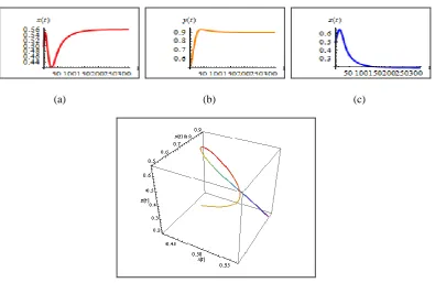
Case 1: m0.108. _{Initially there are large oscillations, which then decrease in size}

very quickly to point equilibrium. Initially the value of m is very small which

means that large number of prey is outside the refuge, so the predator can attack

them quickly and this leads to sharp decrease in prey while the predator grows

rapidly. As a result, the predator population decreases because lacks of food while

the prey increase, but slowly. This cycle is repeated and is faster than previously

but of smaller size. This shows it going to point equilibrium as in figure 1(a, b, c, d)

(a) (b) (c)

Case 2: when m0.5we show there is little oscillations because



1 0.5 0.5



mean the amount of prey is less than the first case and also tends to equilibrium as

Figure 2 (a, b, c, d)

(a) (b) (c)

Figure 2 (the behavior reached the equilibrium)

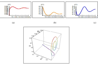
Case 3: Increasing m to become m 0.85 shows sizeable oscillations that go to

the equilibrium. The number of prey outside the refuge is small, the predator

in the initial attack but after that the prey need more time to increasing and when

prey increasing the predator attack them and continuous but weak vibration and

become a limit cycle around equilibrium point figure 3(a, b, c, d)

Figure 3 (low density prey indeed to the limit cyclic)

Second we study the random refuge. To keep all population survive we fixed the

parameters as



r0.5,a0.4,b0.3, 0.08, q10.1,q2 0.0125)and show the

following

Case 1: m=0.02 in this case the



x m



is good quality food to predator so the

predator attack it therefore the prey decreasing and predator increasing and same

as case 1 of system (1) see figures 3 (a, b, c, d).

(a) (b) (c)

Figure 4 (high density of prey in refuge, the behavior reached the equilibrium)

Case 2: increase m tom0.8, in this case the prey outside the refuge is very little so

first and recur more quickly and in a volume less than go in order to form the

orbits around the equilibrium .see figure 4(a, b, c, d)

(a) (b) (c)

Figure 5 (low density of prey, the behavior as the limit cycle)

From above we can say that when high density of prey outside the refuge, the

behavior of the systems in the initial start from a big oscillations and quickly tend

to small oscillations and the equilibrium. When low density of prey outside the

refuge, the oscillations tend to make circles around the equilibrium. Also we

show that a small m in constant refuge is useful because this value give an

oscillations area satisfying continuous harvesting, all population survive with

increasing susceptible predator, decreasing infected predator and a control on

disease see Fig(1.c). But the area in random refuge does not control disease

because in small m, the infected predator increase and susceptible predator

decrease see Fig (4.b).

Conclusion

In this paper we discussed and analysis model prey predator interaction with

harvesting of predator and prey in refuge. We studied bounded solution, and discussed

equilibriums points with its conditions. Show the role affected constant and

points. In the numerical simulation we noticed behavior of models in the high size of

prey in refuges tend to limit cycle around equilibrium. Finally constant refuge give us

an area where continued harvest, all population survive and also to control the disease,

but the random refuge does not guarantee us control the disease where infected

predator increases while the susceptible predator decreasing.

Acknowledgements

This work was fully supported by School of Mathematical sciences, Universiti Sains

Malaysia, Penang Malaysia.

REFERENCES

[1] Anderson, R., R. May, et al.The invasion, persistence and spread of infectious diseases within animal and plant communities .Philosophical Transactions of the Royal Society of London. B, Biological Sciences., 314(1167) (1986), 533-570.

[2] Azar, C., J. Holmberg, et al. Stability analysis of harvesting in a predator-prey model. Journal of Theoretical Biology., 174(1) (1995), 13-19.

[3] B.M,R.B, Effect of prey refuges on a predator –prey model with a class of functional responses:The role of refuges (218)(2012), 73-79.

[4] Chattopadhyay, J. and O. Arino.A predator-prey model with disease in the prey. Nonlinear analysis ., 36(1999), 747-766.

[5] Chen, L. and F. Chen .Qualitative analysis of a predator-prey model with Holling type II functional response incorporating a constant prey refuge.Nonlinear Analysis: Real World Applications ., 11(1)(2010), 246-252.

[6] Chevé, M., R. Congar, et al. (2010). Resilience and stability of harvested predator-prey systems to infectious diseases in the predator.

[7] Dubey, B., P. Chandra, et al. A model for fishery resource with reserve area. Nonlinear Analysis: Real World Applications., 4(4)( 2003), 625-637.

[9] Haque, M. and E. Venturino.The role of transmissible diseases in the Holling–Tanner predator–prey model. Theoretical Population Biology., 70(3)( 2006), 273-288.

[10] Hassell, M. P. and R. M. May. Stability in insect host-parasite models. The Journal of Animal Ecology., (1973), 693-726.

[11] Hochberg, M. E. and R. D. Holt. Refuge evolution and the population dynamics of coupled host—parasitoid associations. Evolutionary Ecology., 9(6)(1995), 633-661.

[12] Ma, Z., W. Li, et al. Effects of prey refuges on a predator-prey model with a class of functional responses: The role of refuges. Mathematical biosciences., 218(2)( 2009), 73-79.

[13] McNair, J. N. The effects of refuges on predator-prey interactions: a reconsideration. Theoretical Population Biology., 29(1)(1986), 38-63.

[14] Rosenzweig, M. L. and R. H. MacArthur.Graphical representation and stability conditions of predator- prey interactions. American Naturalist., (1963), 209-223.

[15] Ruxton, G.Short term refuge use and stability of predator-prey models. Theoretical Population Biology., 47(1)(1995), 1-17.

[16] S.A.Wuhaib,Y.Abu Hasan, (2012).Apredator Infected Prey Model With Harvesting Of Infected Prey .ICCEMS2012: 59-63

[17] Taylor, R. J. (1984). Predation. CHAPMAN AND HALL, NEW YORK, NY(USA).(1984). [18] Venturino, E. Epidemics in predator–prey models: disease in the predators. Mathematical

Medicine and Biology., 19(3)( 2001), 185-205.