Max Planck Institute for Demographic Research Konrad-Zuse Str. 1, D-18057 Rostock·GERMANY www.demographic-research.org
DEMOGRAPHIC RESEARCH
VOLUME 20, ARTICLE 25, PAGES 599-622
PUBLISHED 03 JUNE 2009
http://www.demographic-research.org/Volumes/Vol20/25/ DOI: 10.4054/DemRes.2009.20.25
Research Article
Graduating the age-specific fertility pattern
using Support Vector Machines
Anastasia Kostaki
Javier M. Moguerza
Alberto Olivares
Stelios Psarakis
c
°2009 Anastasia Kostaki et al.
2 Parametric models of fertility 600
3 Kernel techniques 603
4 Support Vector Machines 605
4.1 Regularization Theory 605
4.2 Geometrical Interpretation of Support Vector Machines 606
5 Results 607
6 Findings 618
Graduating the age-specific fertility pattern
using Support Vector Machines
Anastasia Kostaki1
Javier M. Moguerza2
Alberto Olivares3
Stelios Psarakis4
Abstract
A topic of interest in demographic literature is the graduation of the age-specific fertility pattern. A classical graduation technique extensively used by demographers is to fit para-metric models that accurately reproduce it. Standard non parapara-metric statistical methodol-ogy, as kernels and splines, might alternately be used for this graduation purpose. Support Vector Machines (SVM) is an innovative non parametric methodology that could also be used for fertility graduation purposes. This paper evaluates SVM techniques as tools for graduating fertility rates. To that end, we apply these techniques to empirical age-specific fertility rates from a variety of populations and time periods. Additionally, for comparison reasons we also fit parametric models and kernels to these empirical data sets.
1Department of Statistics, Athens University of Economics and Business. 76, Patission St. 10434, Athens, Greece. E-mail: [email protected]
1. Introduction
Statistical graduation techniques are useful tools in demographic research, producing esti-mations of the true patterns of age-specific demographic rates. Therefore such techniques can serve in order to provide a clear description of the real shape of age-specific patterns and also consequently serve as a clear basis for population projections.
In fertility analysis, in order to estimate the unknown age-specific fertility rates which underlie the empirical measures, some graduation technique can be applied to the latter, under the assumption that the true rates follow a smooth pattern through age. A stan-dard technique used for graduating the empirical rates is to provide a model that presents the age-specific birth rates as a parametric function of age. Modeling fertility curves has attracted the interest of demographers for many years. A variety of parametric models pre-senting the fertility rates as a function of age have been proposed in order to describe the age-specific fertility pattern. Some of them provide nice fits to the one year age-specific fertility rate distribution (Hoem et al. 1981; Peristera and Kostaki 2007). Recently the utilization of non parametric techniques in smoothing problems has gained attention. Al-ternatively, standard non parametric statistical methodology, such as kernels and splines, might also be used for this graduation purpose.
Support Vector Machines (SVM) is a modern non parametric graduation technique that appeared in the mid nineties in the framework of Vapnik’s Statistical Learning Theory (Vapnik 1995; Moguerza and Muñoz 2006). Since SVM techniques have shown very successful results in smoothing noisy data, such as neighbourhood curves (Muñoz and Moguerza 2005) or nonlinear profiles (Moguerza, Muñoz, and Psarakis 2007), they can probably serve as useful tools for fertility graduation purposes too. For this application, SVMs are used as general purpose smoothers that enforce a degree smoothness that is chosen by the modeler.
This work provides an evaluation of the SVM methodology in the context of fertility graduation. In the next section, a review of existing parametric models for fitting fertility data is given. Section 3 provides a brief presentation of kernel techniques, while Section 4 is devoted to a presentation of SVM methodology. Then, in Section 5, the results of our calculations fitting parametric models and applying kernels and SVM to a variety of empirical data sets are presented, while finally, in Section 6, the main findings of our calculations are briefly discussed.
2. Parametric models of fertility
fits to one year age-specific fertility distributions. At the outset a presentation of these models is provided.
The Hadwiger function (Hadwiger 1940; Gilje 1969) is expressed by,
f(x) =ab c ³c x ´3 2 exp n
−b2³c
x+ x
c −2 ´o
,
wherexis the age of the mother at birth anda,b,c are the three parameters to be es-timated. Chandola, Coleman and Horns (1999) argued that the parameters of the model may have a demographic interpretation as follows. Parameterais associated with total fertility, parameterbdetermines the height of the curve, parametercis related to the mean age of motherhood, while the term ab
c is related to the maximum age-specific fertility rate
(or modal age-specific fertility rate).
The Gamma function (Hoem et al. 1981) is given by,
f(x) =R 1
Γ(b)cb(x−d) b−1exp
½ −x−d
c ¾
, for x > d
wheredrepresents the lower age at childbearing, while the parameterRdetermines the level of fertility. The parametersbandchave no direct demographic interpretation, but Hoem et al. (1981) have made substitution using these by the modem, the meanµand the varianceσ2of the density, so thatc=µ−mandb= µ−d
c = σ
2
c2.
The Beta function also proposed by Hoem et al. (1981) is given by the formula,
f(x) =RΓ(A+B)
Γ(A)Γ(B)(β−α)
−(A+B−1)(x−α)A−1(β−x)B−1, for α < x < β.
Its parameters are related to the meanνand the varianceτ2through the relations
B= ½
(ν−α)(β−ν)
τ2 −1
¾ β−ν
β−α and A=B ν−α β−ν.
As Hoem et al. (1981) mention, the parametersαandβ are frequently interpreted as the lower and upper age limits of fertility, respectively. The parameterRdetermines the overall level of fertility.
Schmertmann (2003) proposed an alternative model for representing age-specific fer-tility schedules. This is obtained by defining three index ages that describe the shape of the age-specific fertility using a piecewise quadratic spline function. This model describes the shape of the age-specific fertility rates in terms of the ages at which some certain char-acteristic points are reached;αis the youngest age at which fertility rises above zero,R
The model proposed is given by
f(x) = (
RP4k=0θk(x−tk)2+, α≤x≤β
0 , otherwise.
Knotst0 < t1. . . < t4 fall in the interval between agesαandβ, wheret0 = a, (the
lowest age of childbearing) and(x−tk)+≡max[0, x−tk].
As Schmertmann (2003) mentions the quadratic spline model can be useful for de-scribing the shape of many fertility schedules but it requires thirteen parameters to be estimated, while their meaning is somewhat opaque. Therefore, he constructed a spline model in which the three index ages[α, P, H]determine the shape functionf(x), while the parameterR determines the level of fertility. The reduction of the number of pa-rameters is achieved by determining knot positions from the index ages and by imposing mathematical restrictions so that the spline function mimics common features of the age-specific fertility rates.
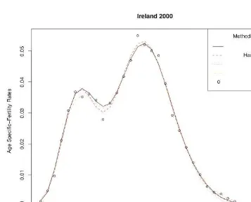
Recently, as Peristera and Kostaki (2007) describe, the fertility pattern in some de-veloped countries exhibits a deviation from its classical shape. Recent data sets of the United Kingdom, Ireland and the USA show distortions in terms of a bulge in fertility rates of younger women. Furthermore, in countries with distorted fertility, the pattern of first births also exhibits an intense hump in younger ages, stronger than that of the total fertility pattern. This heterogeneity initially discovered in the recent fertility distributions of the English speaking European countries and the USA, but recently even in data from other European populations as Spain and Norway, might be related to marital status, re-ligion, educational level and differences in social and economic conditions, as well as to ethnic differences in the timing and the number of births. As expected, the existing mod-els are unable to describe the new shape of the fertility pattern, and therefore the use of more appropriate representations is required.
For describing the new shape of the fertility pattern, Chandola, Coleman and Horns (1999) developed a two-component mixture model of Hadwiger functions which is given by the following expression,
f(x) =am µ b1 c1 ¶µ c1 x ¶3 2 exp ½ −b2 1 µ c1 x + x c1 −2 ¶¾
+ (1−m) µ b2 c2 ¶µ c2 x ¶3 2 exp ½ −b2 2 µ c2 x + x c2 −2 ¶¾ ,
authors, these parameters may also be demographically interpreted. Parameterαis cor-related with the overal fertility level,c1andc2are related to the level and the trend of the
mean ages of births outside and inside marriage.
Recently, Peristera and Kostaki (2007) proposed a flexible model for describing the fertility pattern which in each different version captures both the classical and the distorted fertility pattern. The simpler version of this model (hereafter P-K model) is
f(x) =c1exp
" −
µ x−µ
σ(x) ¶2#
wheref(x)is the age-specific fertility rate at mother agex,c1,µ,σare parameters to
be estimated, whileσ(x) =σ11ifx≤µ, andσ(x) =σ12ifx > µ. The parameterc1
describes the base level of the fertility curve and is associated with the total fertility rate,
µreflects the location of the distribution, i.e. the modal age, whileσ11,σ12reflect the
spread of the distribution before and after its peak, respectively.
An alternative version of this model (hereafter P-K mixture model), which captures the new shape of the fertility pattern mentioned above, is
f(x) =c1exp
" −
µ x−µ1
σ1(x)
¶2#
+c2exp
" −
µ x−µ2
σ2
¶2#
wheref(x)is the age-specific fertility rate at mother agex, whileσ1(x) =σ11ifx≤µ1,
and σ1(x) = σ12 if x > µ1, andc1, c2, µ1, µ2, σ11, σ12, σ2 are parameters to be
estimated.
The parametersc1andc2express the levels of total fertility of the first and the second
hump respectively,µ1andµ2are related to the mean ages of the two subpopulations; the
one with earlier fertility and the other with fertility at later ages. The parametersσ11,σ12
reflect the spread of the distribution of the most intense hump before and after each peak, andσ2reflects the variance of the less intense one.
3. Kernel techniques
Consider a set of observations of two variablesX andY, i.e. data of the form(xi, yi),
i= 1, . . . , pwhich are related via an unknown regression functionmas follows:
yi=m(xi) +εi, i= 1, . . . , p,
where theεiare independent random variables with zero mean and constant variance.
of the neighbourhood over which averaging is performed, called bandwidth, controls the smoothness of the resulting estimator. Hence, an estimator of the functionmof the fol-lowing type is used:
ˆ
mh(x) =n−1
X
Wh(x;X1, X2, . . . , Xn)·Yi,
whereWhis a weight function depending on the bandwidth parameter h and the set of
variablesX1, . . . , Xn.
A conceptually simple approach for the representation of the weight functionWhis to
describe its shape by a density function, called the kernel function, with a scale parameter
h, the bandwidth, that adjusts the size and the form of the weights nearx. Therefore, kernel regression estimators are local weighted averages of the response variable whose weights are determined by the kernel functionK, while the size of the weights depends on the bandwidth parameterh.
Generally, the kernel functionKhas the fundamental properties of a probability den-sity. In the regression context the kernel function is generally a smooth, symmetric, posi-tive function which peaks at zero and decreases monotonically as the bandwidth parame-ters increases in size.
Several formulae have been proposed for the kernel estimatormˆ of the regression mean functionm, depending on the type of the kernel regression estimator used. An ex-tensive presentation of these formulae is provided in Peristera and Kostaki(2005). Among the alternative estimators, Peristera and Kostaki (2005) have shown that the Gasser-Müller estimator (Gasser and Müller 1979, 1984) has proved the most adequate alternative in the context of mortality graduation.
At a pointx, the Gasser-Müller estimator is given by the following formula,
ˆ
mGM(x) = n
X
i=1
Y[i]
Z (x(i+1)+x(i))/2
(x(i)+x(i−1))/2
Kh(x−xi)dx,
wherex0=−∞,xn= +∞,x(i)denotes theith largest value of the observed covariate
values andY[i]is the corresponding response value.
The appropriate selection of the bandwidth parameter is of great importance since it controls the degree of smoothness, and consequently influences the resulting estimator. A presentation of bandwidth selection techniques can be found in Härdle (1990, 1991), and Peristera and Kostaki (2005). An approach for the selection of the bandwidth parameter is to construct a direct plug-in estimator of the optimal smoothing parameterhopt. Gasser,
Kneip and Kohler (1991) give expressions for thehoptappropriate to the Gasser-Müller
one. Local bandwidth selection permits one to obtain a bandwidth that adapts for local efficiency in different parts of the design points, which means that a smaller bandwidth is used in areas of high density while the value of the bandwidth increase in areas of low density. Brockmann, Gasser and Herrmann (1993) and Herrmann (1997) have mentioned the advantage of using kernel regression estimators with a local bandwidth instead of a global one. The main idea of the plug-in method is to estimate the optimal bandwidths by estimating the asymptotically optimal mean integrated squared error bandwidths. For the selection of a local bandwidth, Herrmann (1997) developed an iterative plug-in algorithm that is a generalization of the global iterative plug-in algorithm of Gasser, Kneip and Kohler (1991). A description of this algorithm can be found in Herrmann (1997), in which the advantage of this approach over both the cross-validation method and the global plug-in rule, is highlighted.
4. Support Vector Machines
Support Vector Machines (SVMs) appeared in the middle nineties in the framework of Vapnik’s Statistical Learning Theory (Vapnik 1995; Moguerza and Muñoz 2006), provid-ing very successful results for the smoothprovid-ing of noisy data such as neighbourhood curves (Muñoz and Moguerza 2005) or nonlinear profiles (Moguerza, Muñoz and Psarakis 2007). Support Vector Machines are regularization methods. These methods also include Splines (Moguerza and Muñoz 2006). In fact, there is a close relation between SVM and splines (Pearce and Wand 2006). Next we provide a description of the regression version of SVM and its main features.
4.1 Regularization Theory
Regularization methods (Tikhonov and Arsenin 1977), allow the construction of smooth functions by solving an optimization problem of the form:
min
f∈HK
1 p
p
X
i=1
L(f(xi)−yi) +Mkfk2K,
where(xi, yi), i= 1, . . . , pare a set of data withxi∈Rnandyi∈R,Lis a loss function,
M >0is a constant,HKis a Reproducing Kernel Hilbert Space5(RKHS, see Aronszajn
1950; Moguerza and Muñoz 2006) generated from a kernelK : X ×X −→ R(for instance, the spaceX may be defined asRn), andkfk
K is the norm off in the RKHS.
Notice that, for a fixed value ofz,K(x, z)defines a function ofx. Roughly speaking, a
RKHS is a space made up of linear combinations of functionsK(x, zi), and their limits.
For the case of regression SVM, the loss functionLis defined as:
L(x) = (
|x| −ε, if|x| ≥ε, 0 , otherwise,
whereε > 0is a constant. The idea is to find a smooth functionf∗ ∈ H
K that solves
the optimization problem above. This function, which, as already stated, belongs to the RKHS HK, will have the form f∗(x) =
Pp
i=1αiK(x, xi) +b∗, where αi and
b∗ are constants,K(x, y) = Φ(x)TΦ(y)is the kernel function that generatesH
K and
Φ :Rn −→ Rmis a mapping definingK. In this way, geometrically,Φmaps the data
from the so-called "input space" (that is,Rn) into the "feature space" (that is,Rm). The
constantM >0penalizes non-smoothness of the possible solutions to the problem.
4.2 Geometrical Interpretation of Support Vector Machines
Although the previous formulation is the one that provides the best theoretical properties, from a practical point of view regression SVM can be presented from its geometrical in-terpretation. It can be shown (Moguerza and Muñoz 2006) that the regularization problem can be formulated as a convex quadractic optimization problem (therefore, without local minima) of the form:
min
w,b,ξ,ξ0
1 2kwk
2+C
p
X
i=1
¡ ξi+ξi0
¢
such that ¡wTφ(x i) +b
¢
−yi ≤ε−ξi, i= 1, . . . , p,
yi−
¡
wTφ(xi) +b
¢
≤ε−ξi0, i= 1, . . . , p,
ξi, ξ0i≥0, i= 1, . . . , p,
where ξi and ξi0 are slack variables which permit the violation of a boundary
deter-mined by ε. It can be shown (see Moguerza and Muñoz 2006, for the details) that
f∗(x) = Pp
i=1αiK(x, xi) +b = (w∗)TΦ(x) +b∗, wherew∗ andb∗ are the values
ofwandbat the solution of the quadratic optimization problem. One of the key issues of SVM is how to useφ(x)to map the data into a higher-dimensional space. To achieve this task, a kernel approach is used in order to operate in the feature space without ever computing the coordinates of the data in that space, but rather by simply computing the inner products between the images of all pairs of data in the feature space. Three are the most widely used kernels: the linear kernelK(x, y) = xTy, which corresponds to
constants, which maps the data into a finitely dimensional space; and the Gaussian kernel
K(x, y) = e−kx−ykσ 2, where σ is a positive constant which maps the data into an
in-finitely dimensional space. The Gaussian kernel, given its approximation capacity, is the most extensively used (see Moguerza and Muñoz 2006, for a complete set of examples). In practice, the optimization problem to solve is not the primal formulation shown above. For practical purposes, the problem to solve is the "dual problem" (Schölkopf et al. 2000), that is:
max
λ,λ0 −
1 2
p
X
i,j=1
(λi−λ0i)(λj−λ0j)K(xi, xj)−ε p
X
i=1
(λi−λ0i) + p
X
i=1
yi(λi−λ0i)
such that
p
X
i=1
(λi−λ0i) = 0,
0≤λi≤C, i= 1, . . . , p,
0≤λ0
i≤C, i= 1, . . . , p.
It can be shown that both problems, primal and dual, are equivalent, and that:
f∗(x) =
p
X
i=1
(λ∗
i −λ0∗i )K(x, xi) +b∗= p
X
i=1
αiK(x, xi) +b∗,
whereαi = λ∗i −λ0∗i ,λ∗i andλ0∗i being the values ofλi andλ0i at the solution of the
dual problem. Therefore, in practice, the estimated parameters are the αcoefficients, whose number is p, that is, the number of data. In this way, the relationship between kernels and SVM is clear: only the closed form of the kernelKis needed, and not the explicit mappingΦ. Notice that this distinctive peculiarity allows, for instance, the use of the Gaussian Kernel in order to evaluatef∗(x). Moreover, in practice, only a small
percentage of theαcoefficients will differ from zero, which makes simpler the evaluation of this function (this is one of the advantages of SVM, see Moguerza and Muñoz 2006), and reduces the number of estimated parameters.
5. Results
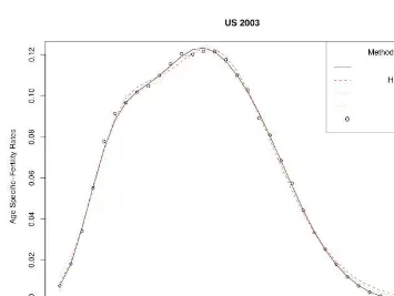
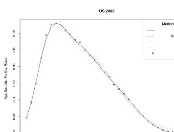
and Ireland 1995 and 2000, as well as for the white and black populations of the USA 2003 and the cohorts of 1942 and 1963 for Spain The empirical data sets were obtained fromEurostat New Cronosdatabase. Additionally, single year age-specific fertility rates for the US were derived from the 2003Natality Data Set, obtained by request from the US National Centre of Health Statistics. Cohort data for Spain for the generations born from 1942 to 1963, obtained from theEurostat New Cronosdatabase. It should be noted that even for cohorts not yet completed,Eurostatprovides estimates of the fertility rates for older women by using the rates observed for previous generations, without waiting for the cohort to reach the end of the reproductive period.
The fits of the parametric models presented at the outset were initially calculated by Peristera and Kostaki (2007). In populations with no apparent early-age hump, the Had-wiger, Gamma, Beta, P-K, and quadratic spline models (Schmertmann 2003) are fitted, while in cases of distorted fertility distributions, the Hadwiger (Chandola, Coleman, and Horns 1999, 2002) and the P-K mixture models ( Peristera and Kostaki 2007) are fitted. The simple models used previously in data sets without distortions had a rather disap-pointing performance in the distored data sets.
In order to avoid heterogeneity we also use data differentiated by order of birth, and cohort and period data sets. Finally in the case of the USA, the fits of the alternative models are provided for the white and black population separately.
In order to fit the alternative parametric models, it is generally accepted that the most efficient procedure is to use weighted least squares, with weights equal to the reciprocals of the variances of the empirical rates. However, as pointed out by Hoem (1976) and Hoem et al. (1981), a weighted estimating procedure would give too much attention to the low fertility ages in the tails and especially to the higher ones in the upper tail, while giving too little attention to the high fertility ages in the middle, and thus is not desirable. Therefore, for the estimation of the parameters of the various models, a non-linear unweighted least-squares procedure is adopted. The models are fitted by means of a Gauss-Newton optimization scheme. The Matlab built-in routine for non-linear parameter estimationlsqnonlinis used in order to find the unconstrained minimum of the unweighted residual sum of squares.
The quadratic Spline estimates are obtained using the program provided by Schmert-mann (2003) at the web page http://mailer.fsu.edu/ schmert/qsfit/qsfit.htm.
by cross-validation leading to a value of 1.9066 for all the estimated curves. In this way, we have a unique model for all the data sets.
For the SVM techniques, the subroutinesvmof the librarye1071for the R-package is used. This is available in http://cran.r-project.org/. A two-step simulation procedure is used to select the parametersε,σandCof theε- regression procedure: εis used to fix the width of a band around the fitted curved,σplays the role of a variance, andCis an upper bound for theλcoefficients in the dual optimization problem and, at the same time, penalizes the values of the slacks corresponding to those points lying outside of the band determined byεin the primal optimization problem. In a first step, the range of parametersε,σandCare determined. Then in a second step, the best combination of the three parameters is computed using R flow sentences. In particular, the values
ε = 0.0001, σ = 40 andC = 1.8, have been chosen for the SVM implementation. Additionally, in this application, the values for the corresponding dimensions in the SVM model aren = 1, m = ∞ (given that this is the dimension induced by the Gaussian kernel, see Moguerza and Muñoz 2006) andp= 34, that is, the number of data within each set. We should notice here again that we use the same set of parameter values for all the data sets. In this way, we are able to make fair comparisons of these results with those produced by kernels.
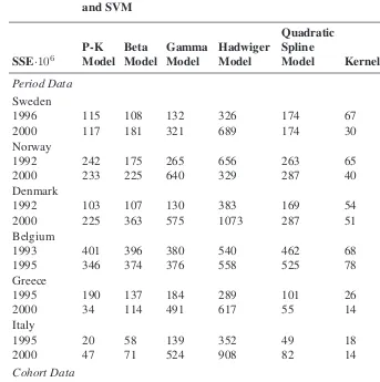
The values of the sums of squares of the differences between the empirical and the resulting values for all the data sets used, and all graduation techniques used, are provided in Tables 1 and 2. The results of fitting the parametric models were first presented in Peristera and Kostaki (2007).
Table 1: Values of the minimization criterion multiplied by 100.000, at the exit of the estimation procedure for P-K model, Beta model, Gamma model, Hadwiger model, quadratic Spline model, kernels and SVM
SSE·106 P-KModel BetaModel GammaModel HadwigerModel
Quadratic Spline
Model Kernel SVM Period Data
Sweden
1996 115 108 132 326 174 67 72
2000 117 181 321 689 174 30 11
Norway
1992 242 175 265 656 263 65 61
2000 233 225 640 329 287 40 10
Denmark
1992 103 107 130 383 169 54 20
2000 225 363 575 1073 287 51 6
Belgium
1993 401 396 380 540 462 68 15
1995 346 374 376 558 525 78 30
Greece
1995 190 137 184 289 101 26 14
2000 34 114 491 617 55 14 13
Italy
1995 20 58 139 352 49 18 11
2000 47 71 524 908 82 14 3
Cohort Data Spain
1943 732 1005 1159 1547 5450 452 562
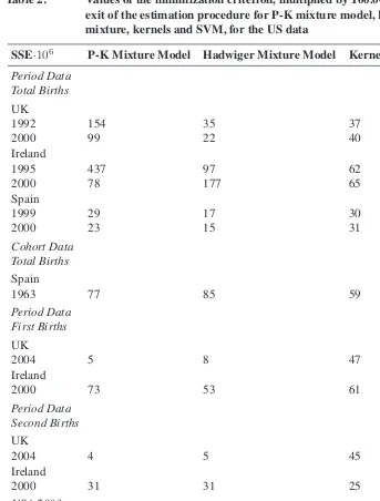
Table 2: Values of the minimization criterion, multiplied by 100.000, at the exit of the estimation procedure for P-K mixture model, Hadwiger mixture, kernels and SVM, for the US data
SSE·106 P-K Mixture Model Hadwiger Mixture Model Kernel SVM
Period Data Total Births UK
1992 154 35 37 14
2000 99 22 40 14
Ireland
1995 437 97 62 90
2000 78 177 65 43
Spain
1999 29 17 30 12
2000 23 15 31 6
Cohort Data Total Births Spain
1963 77 85 59 62
Period Data First Births UK
2004 5 8 47 4
Ireland
2000 73 53 61 62
Period Data Second Births UK
2004 4 5 45 3
Ireland
2000 31 31 25 28
USA 2003
Total 150 28 63 58
White 28 156 63 51
6. Findings
In this paper we propose the application of Support Vector Machines for graduating age-specific fertility rates. In order to evaluate the performance of SVM we apply this tech-nique to a variety of empirical cohort and period data sets of alternative populations. In addition, for comparison reasons, we also fit parametric models and apply kernels to these data sets.
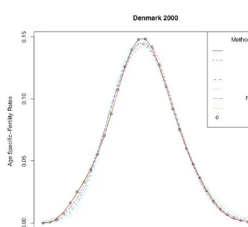
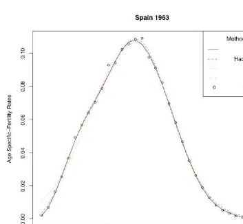
According to the values of the minimizing criterion, the results for the two non para-metric techniques are apparently closer to the empirical values than those provided by the parametric models. This can partly depend on the fact that parametric models provide highest smoothness. A higher degree of smoothness might result from larger distances between the empirical and the graduated values. Turning now to the comparison between the two non parametric techniques, the results provided by the SVM are in most cases associated with lower values of the minimizing criterion.
As is obvious in tables and figures, SVM show a successful performance in graduating the empirical rates in both simple and distorted data sets, producing results that, in the vast majority of cases, are closer to the empirical rates than the other methods. Regarding the figures, one can observe that especially for the ages in the peak and the tails of the fertility curve, the results of SVM were closer to the empirical values than those of most of the other methods.
An advantage of non parametric graduation techniques in comparison with the para-metric modeling is that these can be adequately applied to all data sets, while in data sets with distorted patterns, the use of standard models is inadequate and more complicated formulae are required. Furthermore, the regulation of the degree of smoothness by the user can also be considered as an advantage, allowing the user to choose the optimal de-gree of smoothness depending on the purpose of graduation at hand and also avoiding oversimplification of age patterns.
References
Aronszajn, N. (1950). Theory of reproducing kernels. Trans. Amer. Math. Soc.68: 337– 404. doi: 10.2307/1990404.
Brockmann, M., Gasser, T., and Herrmann, E. (1993). Locally adaptive bandwidth choice for kernel regression estimators. Journal of the American Statistical Associ-ation88(424): 1302–1309. doi: 10.2307/2291270.
Chandola, T., Coleman, D. A., and Horns, R. W. (1999). Recent european fertility pat-terns: fitting curves to ’distorted’ distributions. Population Studies53(3): 317–329. doi: 10.1080/00324720308089.
Chandola, T., Coleman, D. A., and Horns, R. W. (2002). Distinctive features of age-specific fertility profiles in the English-speaking world: Common patterns in Australia, Canada, New Zealand and the United States, 1970-98.Population Studies56: 181–200. doi: 10.1080/00324720215929.
Eurostat New Cronos Database (2006). Europa database:
Popula-tion and Social Conditions (electronic resource). Manchester UK.
http://www.esds.ac.uk/international/support/user_guides/eurostat/Cronoswe.asp. Gasser, T., Kneip, A., and Kohler, W. (1991). A flexible and fast method for automatic
smoothing. Journal of the American Statistical Association86(415): 643–652. doi: 10.2307/2290393.
Gasser, T. and Müller, H. (1979). Kernel estimation of regression functions. In: Smooth-ing Techniques for Curve Estimation. Lecture Notes in Mathematics 757, pp. 23–68. New-York: Springer-Verlag.doi: 10.1007/BFb0098489.
Gasser, T. and Müller, H. G. (1984). Estimating regression functions and their derivatives by the kernel method. Scandinavian Journal of Statistics11: 171–185.
Gilje, E. (1969). Fitting curves to age-specific fertility rates: some examples. Statistical Review of the Swedish National Central Bureau of Statistics III7: 118–134.
Hadwiger, H. (1940). Eine analytische reprodutions-funktion fur biologische gesamtheiten.Skandinavisk Aktuarietidskrift23: 101–113.
Herrmann, E. (1997). Local bandwidth choice in kernel regression estimation.Journal of Computational and Graphical Statistics6(1): 35–54.doi: 10.2307/1390723.
B. (1981). Experiments in modelling recent Danish fertility curves. Demography18: 231–244.doi: 10.2307/2061095.
Härdle, W. (1990).Applied Nonparametric Regression. Cambridge: Cambridge Univer-sity Press.
Härdle, W. (1991).Smoothing Techniques with Implementation in S. New York: Springer-Verlag.
Moguerza, J. and Muñoz, A. (2006). Support vector machines with applications. Statis-tical Science21(3): 322–336. doi: 10.1214/088342306000000493.
Moguerza, J., Muñoz, A., and Psarakis, S. (2007). Monitoring nonlinear profiles using support vector machines. Lecture Notes in Computer Science 4789: 574–583. doi: 10.1007/978-3-540-76725-1_60.
Muñoz, A. and Moguerza, J. (2005). Building smooth neighbourhood kernels via functional data analysis. Lecture Notes in Computer Science 3697: 631–636. doi: 10.1007/11550907.
Pearce, N. and Wand, M. (2006). Penalized splines and reproducing kernel methods.The American Statistician60(3): 233–240. doi: 10.1198/000313006X124541.
Peristera, P. and Kostaki, A. (2005). An evaluation of the performance of kernel estimators for graduating mortality data. Journal of Population Research22(2): 185–197. doi: 10.1007/BF03031828.
Peristera, P. and Kostaki, A. (2007). Modeling fertility in modern populations. Demo-graphic Research16(6): 141–194.
Ruppert, D., Sheather, S. J., and Wand, M. P. (1995). An effective bandwidth selector for local least squares regression. Journal of the American Statistical Association90: 1257–1270.doi: 10.2307/2291516.
Schölkopf, B., Smola, A., Williamson, R., and Bartlett, P. (2000). New support vector algorithms.Neural Computation12: 1207–1245.doi: 10.1162/089976600300015565. Schmertmann, C. P. (2003). A system of model fertility schedules with graphically intuitive parameters. Demographic Research 9(5): 82–110. doi: 10.4054/Dem-Res.2003.9.5.
Tikhonov, A. and Arsenin, V. (1977). Solutions of ill-posed problems. John Wiley and Sons.