doi:10.1155/2010/381953
Review Article
Homology in Electromagnetic Boundary
Value Problems
Matti Pellikka, Saku Suuriniemi, and Lauri Kettunen
Tampere University of Technology, Electromagnetics, P.O. Box 692, 33101 Tampere, Finland
Correspondence should be addressed to Matti Pellikka,[email protected]
Received 4 March 2010; Revised 2 July 2010; Accepted 14 July 2010
Academic Editor: Veli Shakhmurov
Copyrightq2010 Matti Pellikka et al. This is an open access article distributed under the Creative Commons Attribution License, which permits unrestricted use, distribution, and reproduction in any medium, provided the original work is properly cited.
We discuss how homology computation can be exploited in computational electromagnetism. We represent various cellular mesh reduction techniques, which enable the computation of generators of homology spaces in an acceptable time. Furthermore, we show how the generators can be used for setting up and analysis of an electromagnetic boundary value problem. The aim is to provide a rationale for homology computation in electromagnetic modeling software.
1. Introduction
Setting up a well-posed electromagnetic boundary value problem encompasses setting up constraints that are related to the problem domain: the boundary conditions, field sources, and material parameters. These constraints usually surreptitiously involve the topology of the field problem domain. The division of the domain boundary to be governed by different boundary conditions, imposed source fields or circuit quantities, the division of the domain to conducting and nonconducting subdomains, and the use of field potentials bring up topological aspects that cannot be overlooked when defining the boundary value problem
1–6.
Failure to provide the above information in a consistent manner often leads to an over-or underdetermined system, and wover-orse than that, the user as well as the software might be clueless where the problem lies. In this light, an automated, fast and definite procedure to find out the keystones of problem topology would save human effort and supersede problem-specific methods and heuristics in EM modeling software.
boundary value problem domain, while the relative homology is needed when the boundary values are imposed for the unknown fields, or the boundary value problem is coupled to external systems.
In this paper, we represent a succession of algorithms that, when given a cellular mesh, will lead to computation of generators of homology groups in an acceptable time and memory, establishing the viability of homology computation as an integral part of an electromagnetic modeling software. We also discuss how the information provided by homology computation can be exploited.
2. Homology
The study of homology is sewed around the concept of boundaryof a chain, which is an intrinsic part of Maxwell’s integral equations and Stokes’ theorem. We define a boundary operatoron chains, which maps chains to their boundary chains. A chain with zero boundary is called a cycle, and the boundary of the boundary of any chain is empty. Therefore, all boundaries are cycles. However, the converse is not true, there can be cycles that are not boundaries. This makes a dramatic difference in the integration of closed fields over cycles. By Stokes’ theorem, the integrals of closed fields vanish over boundaries, but not necessarily over cycles. Therefore, if two cycles differ only by a boundary, integrals of closed fields over them are equal, and they can be considered equivalent in this sense. Thehomology spacesthey are generalizable intomoduli, but we restrict to spaces with coefficient field ofRorC, which are sufficient to our applicationof achain complexprovide reliable means to classify cycles depending on their contribution to the integrals of closed fields. The elements of homology spaces are thuscosetsof cycles.
To algebraize the concepts of boundary and chain, we form a finitely generated chain complexCKbased on a cellular meshKof the problem domain Ω. The cellular meshK is an instance of theregular cell complex, a finite element mesh for example. The domainΩis taken to be anorientable manifold with boundary. Now, the finite spaces ofp-chains constitute a chain complexChain complex: im∂p 1⊂ker∂pfor eachp. under the boundary operator.
It is represented by an incidence matrix∂p, one for each dimensionp. If we chose to disregard
part of the chains that lie in a subdomainΓ ⊂∂Ω, covered by cell subcomplexL, we get so-calledrelative chain complexCK, L 5,7.In a case boundary values of the unknown field are imposed Γ ⊂ ∂Ω, we are not interested about the field integrals there. This is done by forming an inclusion mapi : CL → CKand quotienting to get CK/iCL. In boundary value problem, the quotient can be formed by dropping the rows and columns from ∂p corresponding to elementaryp-chains that lie inLAs there are no boundary conditions
concerning a multiplicity of a boundary, this is a practical choice of representatives for the relative chains ofCpΩ,Γ.IfLis empty, we call the chain complexabsolute. Our discussion
applies to absolute homology as well. Also, the distinction between the domainsΩ,Γand the FE meshesK,Lis disregarded, andΩandΓare used throughout.Chain spaceCpK, Lis
finite dimensional whereasCpΩ,Γis not, whileHpK, LHpΩ,Γ.
2.1. Decomposition of Chains and Cohomology
It holds that for eachp, the relativep-chain space has the nonunique decomposition5
That is, a nonzero relative chain is a relative boundary of somep 1 chain, that it belongs to an equivalence class of chains that are neither boundaries ofp 1 relative chains and do not have a relative boundary in the chain spaceCp−1Ω,Γ, or it is a relative chain that has a
nonzero relative boundary. SpacesBpΩ,ΓandHpΩ,Γconstitute a space ofp-chains whose
boundaries are empty, the relativep-cyclesZpΩ,Γ.
It turns out that the relative homology spaces, moduli in general, HpΩ,Γ are
interesting when posing an electromagnetic boundary value problem.Restriction to space disregards torsion, which may occur in relative homology of orientable manifolds 7. Our implementation uses integer computations to detect it.They are isomorphic withcohomology spacesHpΩ,Γof therelativecochainsCpΩ,Γ. Cohomology is constructed on theexterior
derivative,in our context of the de Rham cohomology, d in the similar manner homology concerns the boundary operator1,9.In general, this operator is calledcoboundary operator. Cochains can be used to model the electromagnetic fields, and the integration of fields can be regarded as a bilinear mapping : CpΩ,Γ×CpΩ,Γ → Rof chains and cochains1,9.
The subdomainΓ⊂∂Ωis typically a region where a boundary condition is imposed upon an unknown field.
Cohomology and homology are related by de Rham’s theorem. A fieldω ∈ CpΩ,Γ
isclosedif dω 0, andexactifω dαholds. By de Rham’s theorem, a fieldω∈ CpΩ,Γis
exact if and only if
dω0,
c
ω0, ∀c∈HpΩ,Γ. 2.2
Fields that are closed but fail to be exact belong to the cohomology classHpΩ,Γ. Now, such
fields can only exist if the homology spaceHpΩ,Γcontains nonzero elements. Otherwise by
2.2and Stokes’ theorem, all closed fields are also exact. This isde Rham isomorphismbetween homology and cohomology:HpΩ,ΓHpΩ,Γfor allp9. Therefore, computation of the
relative homology of the boundary value problem domain gives us full understanding of how the boundary conditions fix the cohomology classes of the unknown fields, what is left to be determined because of tunnels or voids in the domain.
2.2. Some Properties and Examples of Homology Spaces
The relation between absolute and relative homology spaces can be summarized with the exact sequence of homology spaces1:
· · · −→HpΓ−→i∗ HpΩ j∗
−→HpΩ,Γ ∂p
−−→Hp−1Γ−→ · · ·. 2.3
Here i∗ and j∗ are an inclusion and a projection induced by the corresponding mappings of chain spaces 5,7. That is, all the elements ofHpΩ,Γ can be decomposed into such
nonunique parts that either have a nonzero preimage in HpΩor image in Hp−1Γ. This
twofold structure ofHpΩ,Γemerges when the domainΩcontains tunnels or voids, where
field sources might be present in electromagnetic boundary value problem. Such sources can be taken into account with the aid of generators ofHpΩ,Γ, which have a counterpart in
α
γ
β ζ
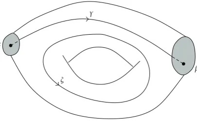
Figure 1:Two representatives of generators ofH1Ω,Γ. One generator has a nonzero preimage inH1Ω,
while the other has image inH0Γ.
Example 2.1. A toroidΩwhereΓconsists of the two shaded walls in is shown Figure1. 1-chain cosetsγandζgenerateH1Ω,Γ. Generatorζhas a nonzero preimage inH1Ω, while generatorγhas image inH0Γ:β−α.
LetΩbe ann-dimensional manifold. Then there exists an isomorphism1,9
HpΩHn−pΩ, ∂Ω. 2.4
If the boundary∂Ωis divided into two complementary nonoverlapping partsΓ1andΓ2, there exists an isomorphism1,9
HpΩ,Γ1Hn−pΩ,Γ2. 2.5
These are so-called duality theorems, actually, compositions of the Lefschetz and de Rham duality theorems1,9,It is crucial that the coefficient fields are the same on the homology and cohomology side., which turn out to be useful together with the isomorphism between chains and cochains when considering dual formulations of an electromagnetic boundary value problem.
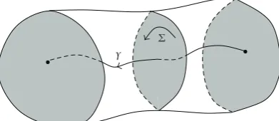
Example 2.2. Dual generators of a barΩin are shown Figure 2.Γ1 consists of the opposite shaded ends of the tube, andΓ2 consists of the jacket. 1-chain cosetγgeneratesH1Ω,Γ1, while 2-chain cosetΣgenerates the dual spaceH2Ω,Γ2.
3. Computation
γ Σ
Figure 2:Representatives of dual generators.
The computation of the p: th homology space is about finding the quotient space ker∂p/im∂p 1. In other words, the p: th relative homology-space is HpΩ,Γ
ZpΩ,Γ/BpΩ,Γ. The computation of a basis of this quotient space using the bases forCp
andCp 1can be done with integer matrix decompositions of the boundary operator matrices,
as discussed in7,8. The decompositions are called Hermite normal form and Smith normal form. The problem is divided into three parts: finding bases for ker∂pand im∂p 1, finding
an inclusion mapi: im∂p 1 → ker∂p, and finding a basis for quotient ker∂p/iim∂p 1.
Unfortunately, the computation of the relevant integer matrix decompositions has worse thanOmaxNp, Np 13upper bound for computational time complexity, whereNp
is the number ofp-cells in the complex10. This is unacceptable, as finite element solution of a boundary value problem is a lot cheaper. However, the number of generators ofHpΩ,Γ
is practically always substantially smaller thanNp, which suggests that we need to look for
means to reduce the size of the bases ofp-chain spaces without altering the relative homology spaces. Only after that, the integer matrix decompositions of the reduced boundary operator matrices are used to compute the generators of homology spaces.
3.1. Problem Size Reduction
Homology spaces are topological invariants and they are isomorphic underweak homotopy equivalences 7, 11, 12. Those properties provide that homeomorphisms and homotopy invariant mappings between topological spaces also preserve the homology spaces. Therefore, it is possible to apply certain homotopical operations to the problem domainΩ, which keep the homology spaces HpΩ,Γ invariant. When the domainΩis covered by a
regular cell complexC, two operations of this kind can easily be exploited7,13as follows.
iFirst is removing a cell that bounds only one cell, together with the cell it bounds. This makes a dent in the domain but not any holes. The corresponding homotopy invariant mapping of the underlying spaceΩ, is called deformation retraction12. In13, this is referred to asexterior face collapsing.
iiSecond is combining neighboringp-cells that share on their boundary a common p−1-cell that is not bounding any otherp-cells. This mapping leavesΩintact. It only alters the chain complexC, which still covers the same domain. Therefore, the topology ofΩdoesnot change. In13, this is referred to asinterior face reduction.
C:cell complex
Repeat
for allp−1-cellscp−1∈Cdo
ifcp−1is on the boundary of exactly onep-cellcpand cp, cp−1∈Ω\Γorcp, cp−1∈Γthen
C:C\ {cp−1, cp} end if
end for
untilno cell has been removed
Algorithm 1:p-Reduce.
nonlocal reduction methods in order to avoid algebraic computations until the sizes of the bases ofp-chain spaces are modest. The reason we split the reduction techniques in13in two separate algorithms is that the former alone is found more computationally efficient, and one should only after that resort to the latter.
3.1.1. Reduction of Cells
If ap-cellcphas a boundaryp−1-cellcp−1that does not bound any otherp-cell, both of these
cells can be removed from the cell complex without altering the relative homology spaces HpΩ,Γ 7,13. These cell pairscp−1, cpsatisfying the above condition are calledelementary
reduction pairs. LetNpbe the number ofp-cells in the cell complexC.
An estimate for the computational complexity Algorithm 1 is in our interest. The order in which the cells are removed affects the efficiency of the algorithm, which ultimately depends on the index numbering of the cells. It is possible to construct examples where the repeat-until-loop must be ran maxNp, Np−1times, resulting to at least quadratic worst case
computational complexity. However, for a typical manifold of a boundary value problem, the loop runs only a couple of times. That gives us more promising estimate when the cell complexCis implemented as a binary search tree and the cells carry the information about their boundary cells. The computational complexity is then essentially due to the linear-time for-loop and the logarithmic-time operation of removing items from a binary search tree. This estimate isONp−1logmaxNp, Np−1.
The removal of ap- and ap−1-cell corresponds to the removal of a row and a column from the matrix of∂pand the removal of a row from the matrix of∂p−1. The matrix of∂p 1
does not change as the removedp-cell cannot be on the boundary of anyp 1-cell. In such case, nop−1-cell can be found that satisfies the if-clause in the algorithm. The algorithm can be applied to the cell complex in succession from the dimensionnof the cell complex down top1. Note though, that the matrix operations are not definitely the most efficient way of implementation.
The number of pairscp−1, cpthe algorithm is able to remove from the cell complex
ranges from zero to all of them. Usually one successful removal triggers an avalanche of removals. Therefore, the cases where no cells can be removed are the most dramatic, and we enumerate the three possible casesFigure3for each connected componentΩi of the
Ω
Σ Θ
Figure 3:Three manifolds: a 3-dimensional tubeΩ, thesurfaceof a toroidΣ ∂Σ ∅, and a solidΘ ∂Θ Γ,
whereΓconsists of the shaded regions. Reduction is able to reduce cells from cell complexCΩ,ΓΩ, but not from complexesCΣandCΘ,ΓΘ.
1∂Ωi/∅,∂Ωi ⊆/Γ: elementary reduction pairscn−1, cncan be found. There existn−
1-cells in∂Ωi\Γthat bound only onen-cell ofΩi;
2∂Ωi∅: no elementary reduction pairscn−1, cncan be found. A manifold without
a boundary: there can be non−1-cells bounding only onen-cell, otherwise they would belong to the boundary;
3∂Ωi⊂Γ: no elementary reduction pairscn−1, cncan be found. This is similar to the
first case, but all then−1-cells in possible elementary reduction pair candidates for removal belong toΓ.
In the last two cases no n−1-cells can be found that satisfy the if-clause in the n-Reduce algorithm. The inability to remove any pairs cn−1, cnimplies that no lower dimensional
pairs can be removed eithertrue for cell complexes whose underlying space is a manifold. It seems thatp-Reduce algorithm is toothless in many situations, but fortunately we can resort to an approach derived from theCoreduction homology algorithm14.
3.1.2. The Reduce-Omit Algorithm
Coreduction, as opposed to reduction, is the procedure of removingp-cell andp−1-cell pairs
cp, cp−1when thep-cellcphas only onep−1-cellcp−1on its boundary. This paircp, cp−1is
called anelementary coreduction pair. As no such pairs can be found from a complete cellular mesh, the algorithm is started by arbitrarily removing a single 0-cell, leaving pairs c1, c0
which satisfy the condition. The algorithm goes on by removing one 0-cell each time there are no elementary coreduction pairscp, cp−1left, while there are still 0-cells left. The number
of arbitrary removals needed to be done in order to banish all 0-cells equals the Betti number β0, the number of connected components of the domain14.
The 0-cell removal is justified by treating the cell complex as thereduced cell complex constituting together with the augmentation map : C0 → Zan augmented chain complex 11., where there is one additional −1-cell in each connected component ofΩ. Thus, the removal of 0-cell is interpreted as the removal of the coreduction pair c0, c−1. For the
reduced homologyhomology for the augmented chain complex, an example of anextraordinary homology theory 11.HC HC\ {c0, c−1} holds14. For the reduced cell complex
H0Ωi 0 holds for each connected component, and HpΩ HpΩ holds for allp /0
11. The information lost aboutH0Ωdue to computing the reduced homology instead can be recovered by storing the arbitrarily removed 0-cells: they are the generators ofH0Ω.
The algebraic dual of a cellular mesh is a mesh where the roles of the cells in the boundary relation of cells have been interchanged. We sayc1is on the coboundary of cellc2, if c2is on the boundary ofc1. So in the dual mesh, boundary cells of a cell become coboundary
the manifold isn, the dual cell of ap-cell is ann−p-cell. For the dual mesh, the boundary operator matrices are∂p ∂Tn−pfor eachp, that is, the transposes of the boundary operators
of the primal mesh5.
Coreduction is a dual algorithm to reduction in the sense that, instead of checking whether ap−1-cell is on the boundary of a singlep-cell only, it checks whether ap-cell is on the coboundary of a singlep−1-cell only.So the Coreduction can be interpreted as a reduction algorithm for the dual mesh in terms of primal mesh cells. Due to the isomorphism between primal and dual cells, the coreductions can be regarded as weak homotopy equivalences.
A dual version of the launch of the Coreduction can be used to devise an extension to p-Reduce algorithm, butonlyin the casepequalsn: Applying the arbitrary removal ton-cells from the cell complex each time it notices no elementary reduction pairscn−1, cncould be
found in the previous run, yet there still aren-cells left. The three cases enumerated earlier tell us that this is the case only when∂Ωi is either empty or a subset ofΓ. The p-Reduce
algorithm detects this nonexistence of elementary reduction pairs in linear time. Similarly to the Coreduction, the number of arbitrary removals needed to banish all then-cells from the cell complex tells us the dimension ofHnΩ,Γ, the Betti numberβn. By duality theorem
HnΩi, ∂ΩiH0Ωi,βnis equal to the number of connected componentsΩiofΩ, for which
either∂Ωi∅or∂Ωi⊂Γholds.
Therefore, each arbitrary removal of an-cell leads to a removal of all then-cells in the given connected component ofΩand the removedn-cells together with the “trigger”n-cell constitute a generator ofHnΩ,Γ. This procedure of course leaves then-generators out of
the final algebraic problem and without orientation, but they can be recovered afterwards. The operation also clearly alters the topology of the domain, but in a controlled fashion. It is known exactly how many and whichn-generators were omitted: one for each connected componentΩiofΩ, for which either∂Ωi∅or∂Ωi ⊂Γholds. We call Algorithm2
Reduce-Omit.
This strategy cannot be applied further down in the dimension p < n, as there is no guarantee that thep-generators have separate supports. Therefore, the arbitrary removal of a p-cell could lead to a removal of such set of p-cells, from which no representative of the generator ofHpΩ,Γcan be constructed. The dimension nwas exceptional, as all the
n-generators had separate supports, and therefore all the removed n-cells constituted one n-generator. For this reason, it seems that the power of the Coreduction algorithm in Betti number computations does not carry over to homology generator computation.
3.1.3. Combining Cells
If ap−1-cell resides on the boundary of exactly twop-cells, it is possible to combine these two p-cells to form singlep-cell and remove thep−1-cell from the cell complex without altering the covered domainΩ.7,13.
Algorithm 3 has worst-case computational complexity ofONpNp−1, where Np is
C:cell complex
n:dimension of the cell complexC βn:0
forpnto 1do
p-ReduceC, p
end for
whilecell complexChasn-cellscnsuch thatcn∈Ω\Γdo
choosen-cellcn∈Csuch thatcn/∈Γ
C:C\ {cn}
βn:βn 1
forpnto 1do
p-ReduceC,p end for
storecnandn-cells removed byp-ReduceC,nin previous loop. end while
Algorithm 2:Reduce-Omit.
C:cell complex
Q:empty queue ofp−1-cells
for allp-cellscp∈Cdo
enqueue boundaryp−1-cells ofcpintoQ
whileQis not emptydo
dequeuecp−1fromQ
Ifcp−1is on the boundary of exactly twop-cellsc1p,cp2and c1
p,c2p,cp−1∈Ω\Γorc1p,c2p,cp−1∈Γthen C:C\ {cp−1, c2p}
c1
p:c1p±c2p, the sign chosen such that the orientations match
enqueue boundaryp−1-cells ofc1
pnot already inQtoQ end if
end while end for
Algorithm 3:p-Combine.
logarithmic time by maintaining a binary search tree of the elements in the queue. Again, the end-state of the algorithm ultimately depends on the index numbering of the mesh vertices.
The combining of twop-cells and removal of ap−1-cell correspond to an addition row-operation of two rows followed by removal of a row and a column in the matrix of∂p,
an addition column operation of two columns followed by removal of a column in the matrix of ∂p 1 and a removal of a row in the matrix of ∂p−1. Again, matrix operations are not an
efficient way to reduce the mesh.
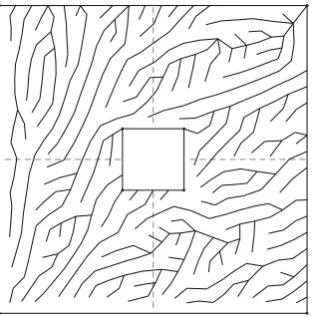
Figure 4:A mesh of a square with a hole after cell combining. Loose tails are left behind, which can be removed withp-Reduce algorithm.
3.2. General Procedure for Homology Computation
Let us now propose a general procedure to find the generators of homology spacesHpΩ,Γ
for allp. Letnbe the dimension of the chain complex.
1Run Reduce-Omit.
2Runp-Combine followed byp-ReduceC,p−1for eachpn−1, . . . ,1.
3Find the generators ofHpΩ,Γusing the reduced boundary operator matrices∂p
for eachpby HNF and SNF.
4Recover the possible generators ofHnΩ,Γfrom the cells stored by Reduce-Omit
optional.
An implementation of this procedure is available in the open source finite element pre- and postprocessor Gmsh15.
3.2.1. Performance Discussion
The total computational complexity of the procedure above quite plausibly depends on the sizes and the ranks of the homology spaces, along with the index numbering of the mesh. Therefore, it is hard to give any definite estimates other than the complexities for individual algorithms in it. However, the upper and lower bounds can be given.
The ultimate upper bound is the computational complexity bound of the Smith normal form decomposition applied to the nonreduced problem10. However, it is highly unlikely that such situation will ever occur in practice with finite element mesh and homology groups without torsion. The worst-case end-states ofp-Reduce andp-Combine are extremely difficult to discover, as they are homotopy invariances, and homotopy groups are known to be computationally challenging. In case the ranks of the homology spaces are zero for all pn, n−1, . . . ,1, the procedure has the computational complexity ofp-Reduce.
a b
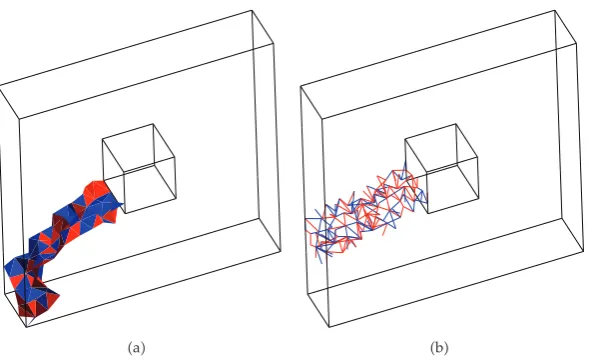
Figure 5:a: A representative of the generator ofH2Ω, ∂Ωof a toroid.b: A representative of the same
generator but in terms of primal mesh cells, so-called thick-cut, computed by applying coreduction to
CΩ.
p-Combine. In case only the ranks of the homology spaces are of interest, the Coreduction homology algorithm can be applied 14. It has the superior computational complexity of ONlogN, whereNis the total number of cells in the cell complex.
3.2.2. A Strategy for Thick-Cuts
Coreduction was found to be a powerful tool to compute the Betti numbers of a cellular mesh, but the answer to whether it is suitable for computation of the generators of homology spaces, seems to be unfortunate. Whenp < n holds, the supports of the generators may overlap, because the recovery of the orientations of the generators iscomplexity theoretically intractable in general7. However, a modified algorithm can be applied to compute the generators, but in no less computational complexity than the reduction algorithm can.
One can apply Coreduction to the cellular mesh so that only 0-cells are arbitrarily removed in a similar but dual manner as in the Reduce-Omit algorithm. Then use straightforward dual versions of p-Combine and p-Reduce. Replace “boundary” with “coboundary” and “p−1-cell” with “p 1-cell” in Algorithms3and1. After that, the homology computation with the reduced andtransposedboundary operator matrices will find out the dual generators of the homology spaces, but in terms of primal cells. An example of this is so-called thick-cut, which we shall discuss more later.
Example 3.1. The established method for finding the generators of HpΩ, ∂Ω is to apply
Reduce-Omit andp-Combine toCΩ, ∂Ωand then compute the decompositions of∂pand
∂p 1. Alternatively, one can apply this modified coreduction technique toCΩ, asHpΩ
Hn−pΩ, ∂Ω holds. Then compute the decompositions of∂Tn−p and ∂Tn−p−1 to find the same
4. Uses
In this section we motivate the interest of computational electromagnetics community in homology computation. The purpose is to show its benefits in an electromagnetic modeling software.
Homology often relates to the electromagnetic phenomena outside the domain Ω, when we want to couple them with the electromagnetic fields defined on the domain. In contrast, modeling decisions are also made to barricade certain kinds of coupling with the outside world. Nevertheless, the interface is always present, and its homological character is an intrinsic part of an electromagnetic boundary value problem.
Before the understanding of the role of homology and cohomology in electromagnetic modeling, case-specific and limited solutions have been used as substitutes. The genuine use of homology can offer a generally applicable and systematic framework for electromagnetic modeling and computation.
4.1. Setting up an Electromagnetic Boundary Value Problem
Setting up an electromagnetic boundary value problem with unique solution involves a variety of questions that, in general, are about the sources of the electromagnetic fields modeled. How does one set the field sources in Ωtogether with the boundary conditions consistently? What does imposing a voltage between terminals actually mean? How does one impose a net current through a conducting domain that has terminals on the domain boundaryΓ? Given multiple terminals, how many and which voltages/currents does one need to impose in order to get a unique solution? When is a field potential sufficient to describe alone the unknown field in electromagnetic boundary value problem?
In simple problems, the above questions can be answered with reasoning based on knowledge about Maxwell’s integral equations and circuit theory. But what if the problem at hand was so complex that simple reasoning would not help or if we wanted to automate the problem posing and validation in order to save human effort. Of course, the software cannot tell what the user wants, but it can help the user to do what he wants as soon as he tells it.
With the aid of homology computation, the software’s answer to all of the above questions would be something like “Impose N of these integrals of these field quantities over these generators of homology spaces in order to get a unique solution.” Next we will present some tangible examples.
4.2. Cuts for Scalar Potential
The use of scalar potential where possible is preferable in field computation, as it reduces the size of the system matrix: there are far less nodes than edges in a typical mesh. Let a closed fieldh∈ Z1Ω {h∈ C1Ω|dh 0}be the field of interest. Due to de Rham’s theorem,
fieldhcan be exhaustively represented with a scalar potentialφ ∈ C0Ωsuch thath dφ
holds, if and only if ch 0 holds for allc ∈ Z1Ω 9. That is, the circulation ofhmust vanish on all closed chains.
Whether this holds for all closed chainscdepends on the homology of the problem domain. It holds by Stokes’ theorem for all chains, that are boundaries, but not all cycles are necessarily boundaries. What is left to be determined are the integrals over nonbounding cycles, valuesIi
c1
c2
S1 S
2
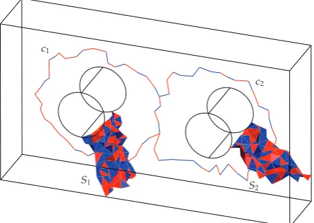
Figure 6:Representativesc1andc2of generators ofH1Ωand the corresponding representativesS1and
S2of the dual generators ofH2Ω, ∂Ω.
homology spaceH1Ω, which is nonempty when the problem domainΩcontains tunnels. However, this fails for a scalar potential alone, as c
idφ
∂ciφ 0 for allci ∈ H1Ω.
Therefore, the fieldhis decomposed into two parts, h dφ T, whereT satisfies dT 0, andc
iT Ii for all ci ∈H1Ω. A systematic approach to fix these circulations forT and
thereby forh, is to produce so-called thick-cuts, where the support ofTentirely lies. This will guarantee sparse system matrix, and the problem is computationally cheap to solve.
There is a multiplicity of methods for finding the thick-cuts. They often mix in homotopy, or rely on some strict assumptions about the domainΩ. However, the cut surfaces are actually the corresponding duals for the generators of H1Ω, elements of H2Ω, ∂Ω, reliably computable with our methods. The thick-cuts are the dual 1-chains of the 2-chain generators ofH2Ω, ∂Ω.
Example 4.1. Consider a magnetic coreΩshaped like Figure8, with coils wound around its branches. The cut surfacesS1andS2, the generators ofH2Ω, ∂Ω, are shown in Figure6.
Example 4.2. Consider a wire wound around a magnetic core that is surrounded by air. LetΩ consist of the core and air, see Figure7. Now, the single generator ofH1Ωis a simple loop around the wire. Its dual generator ofH2Ω, ∂Ωdoes not share this virtue, as it “cuts” all such loops.
4.3. Detection of Contradicting Source Quantities and Boundary Conditions
Figure 7:On the left: a representative of the generator ofH1Ω. On the right, the representative of the
generator ofH2Ω, ∂Ω.
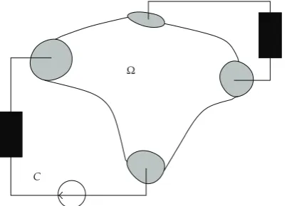
Ω
C
Figure 8:Coupled field-circuit problem. The circuit and field domains are isolated everywhere else except
on the shaded regionΓ⊂∂Ω.
before the solver is launched, to inform the user about possible clashes. For a more detailed discussion, see16.
Example 4.3. Consider a magnetostatic problem where the domainΩ is a current-carrying toroid. The problem is governed by the equations dh j and db 0. The source term j /0 is set inside the domain, and the boundary conditions th f and tb g are set on nonoverlapping regionsΓh,Γb ⊂ ∂Ω, which cover the whole domain boundary. Now, the
magnetostatic equations require that
∂S
h
S
j, ∀S∈C2Ω,
∂V
b0, ∀V ∈C3Ω
Ωc
c3
c2
Ωa
c1
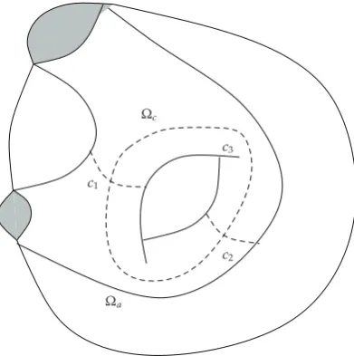
Figure 9: Multiformulational field problem. It is often economical to use different field problem
formulations in the conducting domainΩcand in the nonconducting domainΩa. 1-chain cosetsc1,c2,
andc3generateH1∂Ωc∩∂Ωa.
hold. In order to check whether our boundary conditions comply to those requirements, it is sufficient to check that16
∂s
th
s
j, ∀s∈H2Ω,Γh,
∂v
tb0, ∀v∈H3Ω,Γb,
4.2
where s and v are representatives of the generators of the homology spaces, readily computable with our methods. If the space H2Ω,Γh is not empty and the user has for
example, set th0 onΓhand nonzero net current throughs, then a clash will occur.
This procedure generalizes to all electromagnetic boundary value problems because all of the Maxwell’s equations are of the form
∂c
α
c
ω, 4.3
whereωis the field source, set in the domainΩ\Γ, andαis the unknown field, subject to a boundary condition tαfonΓ. A clash will occur, if∂ctα /cωfor somec∈HpΩ,Γ.
4.4. Setting Up Coupled Circuit-Field Problems
contains no tunnels and subject it to the Kirchhoff’s current law:∂Ωj 0. The state variables of the circuit problem are voltages and currents, which describe the power in the system. The circuit problem and the field problem are isolated in such manner that the field problem constitutes a circuit element. The interfaces between the circuit and the field problem are the conductor terminals onΓ ⊂∂Ω. All the power flux by voltages and currents betweenC andΩis accounted by this interface only, on which voltage and current must have a precise meaning. The isolation is built by boundary conditions
te0, onΓ,
td0, on∂Ω,
tb0, on∂Ω,
tj0, on∂Ω\Γ.
4.4
That is, no magnetic or electric flux passes through the boundary∂Ω, and current can only pass through the terminalsΓ. By tb 0 on∂Ω we are guaranteed to have scalar potential there. TerminalsΓmust be equipotential surfaces to be eligible nodes of the circuit. In order to get an unique solution for the field problem, one needs to set a number of voltages between the terminals and/or currents through them. These constraints are either the state variables of the circuit problem, or preset variables17.
The generators of the relative homology spaces can be used to interpret the coupling through the terminals on the field problem side. Imposing field integrals along the generators corresponds to providing enough information to construct an impedance matrix of the field problem. We will represent two examples where this is intuitively clear. However, homology computation can bring this “intuition” to the computer, and aid the human intuition in more complex problems. It can tell exactly how many “nonlocal” constraints are needed, and the visualizations of the generators help to understand their meaning.
Example 4.4. Consider a DC resistor model in Figure 2 with conducting region Ω, two terminals onΓand an insulating surface∂Ω\Γ. By intuition and experience, one can tell that a unique solution is found by imposing a voltage differenceV between the terminals. In terms of homology, that is, the integral of electric fieldealong the single generatorγofH1Ω,Γ:
γe V. This reveals that we are actually interested in the EMF between the terminals, and
the familiar scalar potential is just one way to impose it. This widens the understanding of the situation beyond the cases where the existence of a scalar potential can be guaranteed everywhere inΩ. However, in coupled field-circuit problems, the scalar potential must exist on the surface∂Ω.
Alternatively, instead of the voltage between the terminals, one can set the net currentI through the resistor. Again, in the language of homology, this is the integral of current density jover the single generatorΣofH2Ω,Ω\Γ, which is the dual generator ofγ. So the user needs to setΣj I. This together with dj 0 guarantees thatΓj 0 will hold. If neither or both the voltage and the net current are set, one is left with an under/over-determined system with no unique solution2, about which homology-aware software is able to inform the user.
and nonconducting regions. Not all terminals are necessarily galvanically connected to each other. Now we can find three generators ofH1Ω,ΓandH2Ω, ∂Ω\Γ, respectively. Imposing voltages between the terminals onΓcorresponds to imposing EMFs along the generators of H1Ω,Γ.
More interestingly, imposing integral of j ∂td over generators of H2Ω, ∂Ω\ Γ
corresponds to imposing currents through terminals, as no displacement current∂tdescapes
from Ω and the continuity equation ∂vj ∂td 0 must hold for all volumes v inside
Ω. Conversely, imposing currents through terminals may impose displacement currents in nonconducting parts of the domainΩ, as well as currents in conducting parts. Homology-aware software would be able to help the user to perceive what has been imposed. In total, three EMFs or fluxes ofj ∂tdmust be imposed to get an unique solution to the problem.
4.5. Multiformulational Field Problem
In many problems, it is possible to use computationally more efficient formulations in some parts the computational domainΩ. For example, the conducting and nonconducting parts of the domain can be treated separately. However, the price for the computational efficiency is the increased effort to set up the problem, as the coupling between the subdomains must be taken into account.
Example 4.6. Let the domainΩconsist of a conducting subdomain Ωc and nonconducting
subdomainΩa. InΩc, we can either have an imposed time-varying source current, or it can
be coupled to an external circuit through terminals on Γ ⊂ ∂Ωc, as described in previous
section. However, letΩahave tunnels, through which the conducting domainΩcextends.
Now, in the air regionΩa, we seek for the solution of the magnetic fieldhonly, for
which dh 0 holds. We are able to use a scalar potential formulation with the thick-cut technique, with expressionhTa dφa. But what should be the total currentsIithrough the
holes in regionΩa, fixing the circulations
cih
ciTa , ci∈H1∂Ωc∩∂Ωa?
In the conductor region Ωc, in addition to the magnetic field, we are interested in
the electric field and the corresponding currents. Therefore, we look for the solution of the
coupled magnetoquasistatic problem defined there. In other words, dh j, db 0, and de ∂tb 0 must hold, where j consists of imposed source current and eddy currents
generated by the time-varying magnetic flux, and tj 0 on∂Ωc∩∂Ωa. The problem is solved
by decompositionhTc dφc inΩc, and on∂Ωc∩∂Ωaby settingφa φcand outside the
thick-cutstTc06. We note that the required currents
Ii
si
j
si
dTc
∂si
Tc
∂si
Ta, si∈H2Ωc, ∂Ωc∩∂Ωa, 4.5
which are also the independent currents of the coupled problem, as∂Ωc∩∂Ωa∂Ωc\Γ.
5. Conclusions
the benefits of homology computation to electromagnetic modeling were discussed. It was suggested that the homology computation, when efficiently implemented, can be a useful preprocessing aid in electromagnetic modeling software. It can be used as a problem posing companion as well as a guardian of the solver, reducing the human effort put to the problem. Many engineering problems, solved with methods of computational electromag-netism, fall into predefined problem categories, for which templates are readily available in the software. This is helpful for the engineer, but it also narrows down the class of problems a software is able to solve. A minor variant of a commonplace problem can make it unsolvable because of some needless but guiding restriction within the software. Homology computation can help the software designer to give freer hands to the user without reducing the software’s usability.
References
1 P. R. Kotiuga,Hodge decompositions and computational electromagnetics, Ph.D. thesis, Electrical and Computer Engineering, McGill University, Montreal, Canada, 1984.
2 A. Bossavit, “Most general “non-local” boundary conditions for the Maxwell equation in a bounded region,”COMPEL, vol. 19, no. 2, pp. 239–245, 2000.
3 L. Kettunen, “Fields and circuits in computational electromagnetism,”IEEE Transactions on Magnetics, vol. 37, no. 5, pp. 3393–3396, 2001.
4 S. Suuriniemi, T. Tarhasaari, and L. Kettunen, “Generalization of the spanning-tree technique,”IEEE Transactions on Magnetics, vol. 38, no. 2, pp. 525–528, 2002.
5 J. Kangas, Algebraic decompositions in analysis of quasistatic electromagnetic problems, Ph.D. thesis, Department of Electrical Engineering, Tampere University of Technology, Tampere, Finland, 2007.
6 R. Specogna, S. Suuriniemi, and F. Trevisan, “GeometricT-Ωapproach to solve eddy currents coupled to electric circuits,”International Journal for Numerical Methods in Engineering, vol. 74, no. 1, pp. 101– 115, 2008.
7 S. Suuriniemi, Homological computations in electromagnetic modeling, Ph.D. thesis, Department of Electrical Engineering, Tampere University of Technology, Tampere, Finland, 2004.
8 T. Kaczynski, K. Mischaikow, and M. Mrozek, Computational Homology, vol. 157 of Applied Mathematical Sciences, Springer, New York, NY, USA, 2004.
9 P. W. Gross and P. R. Kotiuga,Electromagnetic Theory and Computation: A Topological Approach, vol. 48 ofMathematical Sciences Research Institute Publications, Cambridge University Press, Cambridge, Mass, USA, 2004.
10 C. K. Yap,Fundamental Problems of Algorithmic Algebra, Oxford University Press, New York, NY, USA, 2000.
11 J. R. Munkres,Elements of Algebraic Topology, Perseus Books, Cambridge, Mass, USA, 1984.
12 A. Hatcher,Algebraic Topology, Cambridge University Press, Cambridge, Mass, USA, 2002.
13 T. Kaczy ´nski, M. Mrozek, and M. ´Slusarek, “Homology computation by reduction of chain complexes,”Computers & Mathematics with Applications, vol. 35, no. 4, pp. 59–70, 1998.
14 M. Mrozek and B. Batko, “Coreduction homology algorithm,”Discrete and Computational Geometry, vol. 41, pp. 96–118, 2000.
15 C. Geuzaine and J.-F. Remacle, “Gmsh: a 3-D finite element mesh generator with built-in pre- and post-processing facilities,”International Journal for Numerical Methods in Engineering, vol. 79, no. 11, pp. 1309–1331, 2009.
16 S. Suuriniemi, J. Kangas, and L. Kettunen, “Formalization of contradicting source quantities and boundary conditions in quasi-statics,”IEEE Transactions on Magnetics, vol. 43, no. 4, pp. 1253–1256, 2007.