R E S E A R C H
Open Access
A reduced-order extrapolating collocation
spectral method based on POD for the 2D
Sobolev equations
Shiju Jin
1and Zhendong Luo
2**Correspondence:[email protected]
2School of Mathematics and
Physics, North China Electric Power University, Beijing, China Full list of author information is available at the end of the article
Abstract
In this paper, we mainly use a proper orthogonal decomposition (POD) to reduce the order of the coefficient vectors of the solutions for the classical collocation spectral (CS) method of two-dimensional (2D) Sobolev equations. We first establish a reduced-order extrapolating collocation spectral (ROECS) method for 2D Sobolev equations so that the ROECS method includes the same basis functions as the classic CS method and the superiority of the classic CS method. Then we use the matrix means to discuss the existence, stability, and convergence of the ROECS solutions so that the procedure of theoretical analysis becomes very concise. Lastly, we present two set of numerical examples to validate the effectiveness of theoretical conclusions and to illuminate that the ROECS method is far superior to the classic CS method, which shows that the ROECS method is quite valid to solve Sobolev equations. Therefore, both theory and method of this paper are completely different from the existing reduced-order methods.
MSC: 65N30; 65N12; 65M15
Keywords: Proper orthogonal decomposition; Classic collocation spectral method; Sobolev equations; Reduced-order extrapolating collocation spectral method; Existence, stability, and convergence
1 Introduction
LetΩ⊂R2be an open bounded domain with boundary∂Ω. We consider the following two-dimensional (2D) Sobolev equation:
⎧ ⎪ ⎪ ⎨ ⎪ ⎪ ⎩
ut–εut–γ u=f(x,y,t), (x,y,t)∈Ω×(0,T),
u(x,y,t) =ϕ(x,y,t), (x,y,t)∈∂Ω×(0,T),
u(x,y, 0) =u0(x,y), (x,y)∈Ω,
(1)
whereut =∂u/∂t,u=∂2u/∂x2+∂2u/∂y2,ut=∂2ut/∂x2+∂2ut/∂y2,T represents the
final moment,ε> 0 andγ> 0 are two given constants,f(x,y,t) is the known source item, andu0(x,y) andϕ(x,y,t) are the known initial and boundary values, respectively. For sim-plicity but without loss of generality, we further assume thatϕ(x,y,t) = 0.
The system of Sobolev equations (1) is a class of significant partial differential equations (PDEs) with practical physical background, which favorably simulated many engineering problems (see [1,2]). Particularly, it can be applied to simulate the porous phenomenons (see [3,4]). Nevertheless, in actual applications, Sobolev equations frequently contain in-tricate boundary and initial values, complicated source items, or discontinuous constants. As a result, we cannot generally seek analytic solutions, so that we can only rest upon nu-merical methods.
Currently, finite difference (FD), finite volume element (FVE), finite element (FE), and spectral methods are four famous computational techniques. However, the spectral method gives the highest accuracy among the four computational methods since the un-known functions in the spectral methods are approximated with some sufficiently smooth functions, such as Chebyshev polynomials, trigonometric functions, Legendre polynomi-als, or Jacobi polynomipolynomi-als, whereas the unknown functions in the FVE and FE methods are commonly approximated with some standard polynomials, and the derivatives in the FD scheme are approximated with some difference quotients. The spectral method is com-monly sorted into the collocation spectral (CS) method, Galerkin’s spectral method, and the spectral tau method. It has been applied to settle various PDEs including second-order elliptic, parabolic, hyperbolic, telegraph, and hydromechanical equations (see [5–8]).
However, Sobolev equations are mainly solved with the FD scheme, the FE method, and the FVE method (see, e.g., [3,4,9–14]), except that one-dimensional Sobolev equa-tions have been settled by the Fourier spectral method [15], and 2D Sobolev equaequa-tions have recently been settled by the classic CS method [16]. Though the classic CS method (see [16]) for 2D Sobolev equations can attain higher accuracy than the FD scheme, FE method, and FVE method, it also contains a lot of degrees of freedom (unknowns). In this way, because of the round-off error accumulation in numerical calculations, after several computational steps, there generally occurs a floating-point overflow such that we can-not obtain the desired consequences. Hence, to ensure a sufficiently high precision of the classic CS solutions, the crucial question is how to lessen the unknowns (i.e., degrees of freedom) of the CS method to ease the round-off error accumulation in the calculations, which is also central task in this paper.
Many examples have proven that the proper orthogonal decomposition (POD) can sig-nificantly reduce the order of numerical methods (see [17–20]). It can vastly decrease the degrees of freedom in the numerical methods. It has been applied in many fields includ-ing pattern recognition and signal analysis [21], statistical calculations [22], and computa-tional fluid mechanics [23]. For the past few years, it has successfully been used to the or-der reduction for the Galerkin methods [24,25], the FE methods [26,27], the FD schemes [28–30], the FVE methods [31,32], and the reduced basis methods for PDEs [33–35]. Nevertheless, the existing POD-based reduced-order methods (see [17–27,29–35]) are mostly created with the POD bases produced by the classic solutions at all the time nodes on [0,T], before repeatedly finding the order reduction solutions on the same time nodal points. In fact, they belong to some undesirable repeated computations. To get rid of the repeated computations, several reduced-order extrapolated approaches based on POD have been proposed [36–41].
to reduce the order of the coefficient vectors of the CS solutions for the classic CS method, we construct a ROECS method only holding few degrees of freedom. We employ matrix means to discuss the existence, convergence, and stability of the ROECS solutions so that the theoretical means here becomes very concise. In particular, we only employ the classic CS solutions on the first several time nodal points to form the snapshots, and then we use them to produce the POD bases and create the ROECS format so as to obtain the ROECS solutions on all the time nodal points. Thus, we avoid the repeated computations. Moreover, in this paper, we adopt the error estimates to serve as the suggestion of choice of POD bases. The ROECS format contains both advantages that the POD method can reduce the unknowns and the CS method has higher accuracy, so it is an innovation and development of the existing reduced-order methods.
The main merits of the ROECS method hare the following. First, we only reduce the order of the coefficient vectors of the solutions for the classic CS method by POD and have not altered the basis functions for the classic CS method so that the ROECS method holds simultaneously both virtues that POD can reduce the unknowns and the classic CS method has higher accuracy. Second, the classic CS method is totally different from the Galerkin spectral method, and the Sobolev equations not only include a first-order deriva-tive term of time and two 2nd-order derivaderiva-tive terms of spacial variables but also contain two mixed derivative terms of the first order with respect to time and of the second order with respect to spacial variables, that is, the 2D Sobolev equations are more complex than the hyperbolic and parabolic equations in [42,43]. So the ROECS method is totally differ-ent from the methods in [42,43], but 2D Sobolev equations have some special applications as stated before. Third, we use the matrix means to discuss the existence, convergence, and stability of the ROECS solutions so that theoretical analysis becomes very concise and our theory and methods are totally different from the other existing order reduction meth-ods. Therefore, our method is totally new and superior over the existing order reduction methods.
The rest of this paper is organized the following. In Sect.2, we first retrospect the classic CS format of the 2D Sobolev equations and gain snapshots from the initial few classic CS solutions. Then, in Sect.3, we produce a cluster of POD basis from the snapshots, develop the ROECS format, prove the existence, convergence, and stability of the ROECS solutions by the matrix means, and supply the flow-chart for settling the ROECS format. Next, in Sect.4, we use two sets of numerical examples to illuminate that the ROECS format is distinctly superior to the classic CS model, to validate that the numeric computational conclusions accord with the theoretical ones and that the ROECS format is quite valid to solve Sobolev equations, and to confirm that the ROECS format can greatly lessen the unknowns (i.e., degrees of freedom), the calculation load, the CPU elapsed time, and the required storage volumes in numerical computations. Finally, in Sect.5, we provide the chief conclusions and discussions.
2 The classic CS method for 2D Sobolev equations
Because any bounded closed domainΩinR2can be approximately covered with several rectangles [ai,bi]×[ci,di] (i= 1, 2, . . . ,I), for simplicity and without loss of generality, let
Ω= [a,b]×[c,d]⊂R2. Moreover, using the transformsx= –1 + 2(x–a)/(b–a) andy=
2.1 The variational formulation for the 2D Sobolev equations
The Sobolev spaces and norms used in this paper are standard, whose detailed descrip-tions can be found in [44]. For example, we setω= 1/(1 –x2)(1 –y2), andL2
ω(Ω) denotes
the set of all square-integrable functions onΩequipped with inner product and norm
(u,v)ω=
Ω
uvωdxdy, u0,ω=
Ω
|u|2ωdxdy 1/2
, ∀u,v∈L2ω(Ω),
whereasHωm(Ω) :={u∈L2ω(Ω) :Dαu∈L2ω(Ω), 0≤ |α| ≤m}denotes the weighted Sobolev
space onΩwith the CGL quadrature weight function, equipped with the norm
um,ω=
0≤|α|≤m
Dαu20,ω 1 2 .
Furthermore, setH1
0,ω(Ω) ={u∈Hω1(Ω) :u|∂Ω= 0}, and let · Hl(Hm
ω)be the norm in the space
Hl0,T;Hωm(Ω)≡
v(t)∈Hωm(Ω) :v2Hl(Hm ω)≡
T 0 l i=0 dtdiiv(t)
2
m,ω
dt<∞
.
We consider the following variational formulation for 2D Sobolev equations.
Problem 1 Fort∈(0,T), findu∈H1
0,ω(Ω) such that
⎧ ⎨ ⎩
(ut,v)ω+ε(∇ut,∇v)ω+γ(∇u,∇v)ω= (f,v)ω, ∀v∈H0,1ω(Ω),
u(x,y, 0) =u0(x,y), (x,y)∈Ω. (2)
The following result on the existence, uniqueness, and stability of the generalized solu-tion for Problem1has been provided in [16].
Theorem 2 If f∈L2(0,T;H–1
ω (Ω))and u0∈Hω1(Ω),then there exists a unique generalized
solution for the variational formulation(2)satisfying the following stability:
u1,ω≤ ˜c
u01,ω+fL2(H–1 ω )
, (3)
wherec˜=max{1,ε, 1/(γc2
p)}/min{1,ε},and cpis the Poincaré coefficient.
2.2 The classic CS method for the 2D Sobolev equations
Too solve time-dependent PDEs by the CS format, it is necessary to discretizeutby means
of the difference quotient and spatial variables by means of the CS method. The CS method consists in seeking some approximate solutions at time and spatial nodes. In this paper, we take the Chebyshev–Gauss–Lobatto (CGL) type interpolation points (see [8]) as the space nodes, namely, let{xj}Nj=0and{yk}Nk=0be the space nodes in thexandydirections,
respectively, with
xj= –cos
jπ
N, yk= –cos kπ
where the positive integerNdenotes the number of nodes in a certain direction. For in-tegerK> 0, lett=T/Kbe the time step, that is,Kt=T. We approximateu(x,y,nt) withun, the time derivativeu
tofu(x,y,t) at timetn=ntwith (un+1–un)/t, andun(x,y)
withun
N(x,y), namely,
un(x,y)≈un N(x,y) =
N
j=0
N
k=0 un
N(xj,yk)hj(x)hk(y), 0≤n≤K,
where{hj(x)}Nj=0and{hk(y)}Nj=0are the Lagrange basis polynomials associated with the sets of the CGL points{xj}Nj=0and{yk}Nk=0, respectively.
Define theH1
ω-orthogonal projectionRN:H0,1ω(Ω)→PN, that is, for anyu∈H0,1ω(Ω), it
satisfies
∇(RNu–u),∇v
ω= 0, ∀v∈PN.
Thus,RNhas the following important property (see [8]).
Theorem 3 For any u∈Hωq(Ω)with q≥1,we have
∇RNu0,ω≤ ∇u0,ω, ∂k(RNu–u)0,ω≤CNk–q, 0≤k≤q≤N+ 1,
where C is a general positive constant independent of N andt.
Now, we obtain the following CS format for 2D Sobolev equations.
Problem 4 FindunN∈UN ≡H0,1ω(Ω)∩PNsuch that
⎧ ⎪ ⎪ ⎨ ⎪ ⎪ ⎩
(unN+1–unN,vN)ω+ε(∇unN+1–∇unN,∇vN)ω+γ t(∇unN+1,∇vN)ω
=t(f(tn+1),vN)ω, ∀vN∈UN, 0≤n≤K,
u0N(x,y) =RNu0(x,y), (x,y)∈Ω,
(4)
wheref(tn) =f(x,y,tn).
The result on the existence, uniqueness, stability, and convergence about the CS solu-tions for Problem4is given in [16].
Theorem 5 If f ∈L2(0,T;L2
ω(Ω))and u0∈Hω1(Ω),then there exists a unique series of
solutions un
N∈UN (n= 1, 2, . . . ,K)for the CS format(4)satisfying the following stability:
∇unN20,ω≤ ∇u020,ω+
t γ
n
j=1
f(tj)
2
0,ω, n= 1, 2, . . . ,K. (5)
Furthermore,whent=O(N–1)and solutions of Problem1u(t
n)∈Hωq(Ω) (2≤q≤N+ 1),
the errors between the solution for Problem1and the series of solutions of Problem4have the following estimates:
∇
u(tn) –unN0,ω≤C
u(tn) –unN0,ω≤C
t2+N–q, n= 1, 2, . . . ,K. (7) Remark1 The error estimates in Theorem5attain an optimal order. Theorem5shows that the classic CS format, that is, Problem4for 2D Sobolev equations has a unique se-ries of solutions, which is stable and continuously depends on the initial value and source functions. This theoretically ensures that Problem4is effective and reliable for solving 2D Sobolev equations.
2.3 The matrix representation of the classic CS format
To understand more easily the classic CS format for 2D Sobolev equations, we will rewrite the classic CS format (4) in the matrix form so that it can be easily programmed and com-puted by a computer. LetunNj,k (0≤j,k≤N) denote the spectral approximate values of u(xj,yk,nt), namely
u(x,y,nt)≈unN=
N j=0 N k=0
unNj,khj(x)hk(y). (8)
TakingvN=hm(x)hl(y)∈UN(0≤m,l≤N) in scheme (4), we come to the conclusion
unN+1,vN
ω= N j=0 N k=0
unN+1j,khj(x)hk(y),hm(x)hl(y)
ω,
∇unN+1,∇vN
ω= N j=0 N k=0
unN+1j,khj(x)hk(y),hm(x)hl(y)
ω + N j=0 N k=0
unN+1j,khj(x)hk(y),hm(x)hl(y)
ω.
From Problem4we obtain
Ajm,kl=
hj(x)hk(y),hm(x)hl(y)
ω = N p=0 N q=0
hj(xp)hm(xp)ωphk(yq)hn(yq)ωq, (9)
Bjm,kl=
hj(x)hk(y),hm(x)hl(y)
ω+
hj(x)hk(y),hm(x)hl(y)
ω = N p=0 N q=0
hj(xp)hm(xp)ωphk(yq)hl(yq)ωq
+ N p=0 N q=0
hj(xp)hm(xp)ωphk(yq)hl(yq)ωq, (10)
where 0≤j,m,k,l≤N.
Then we can rewrite the classic CS format (4) for the 2D equations as the following matrix form with (N+ 1)2equations for{unNz}Kn=0:
⎧ ⎨ ⎩
(A+εB+γ tB)Un+1
N =tFn+1+ (A+εB)UnN, 0≤n≤K– 1,
where
A= [Ajm,kl](N+1)2×(N+1)2, B= [Bjm,kl](N+1)2×(N+1)2,
UnN+1=unN+10,0,uNn+11,0, . . . ,unN+1N,0,unN+10,1,unN+11,1, . . . ,unN+1N,1, . . . ,uNn+10,N, . . . ,unN+1N,NT,
Fn+1=F0,0n+1,F1,0n+1, . . . ,FNn+1,0,F0,1n+1, . . . ,FNn+1,1, . . . ,F0,n+1N, . . . ,FNn+1,NT, Fmn+1,l =fxm,yl, (n+ 1)t
, 0≤n≤N– 1,
U0=
u0(x0,y0),u0(x1,y0), . . . ,u0(xN,y0),u0(x0,y1), . . . ,u0(xN,y1), . . . ,
u0(x0,yN), . . . ,u0(xN,yN)
T
.
Remark2 Because the classic CS format adopts the Chebyshev polynomials as basic func-tions, it has a higher accuracy than general numerical methods, such as the FE method, FD scheme, and FVE method, but it also contains as many unknowns as the general nu-merical methods, so that it has to bear a lot of computing load. Thus, reducing the order for the classic CS format is more significative than for other numerical methods. For this purpose, we extract the initialLcoefficient vectorsU1
N,U2N, . . . ,ULN (LK) in the series
of coefficient vectors{Un
N}Kn=1 for the classic CNCS matrix format (11) to form a set of snapshots.
3 The ROECS method based on POD for 2D Sobolev equations
3.1 Formulation of POD basis
We use the set of snapshots obtained by Sect. 2.3 to form a snapshot matrix P = (U1N,U2N, . . . ,ULN) of volume (2N+ 1)2×L. Letλ
j> 0 (j= 1, 2, . . . ,r=:rank(P)) be the positive
eigenvalues ofPPT arranged nonincreasingly, and letU= (φ1,φ2, . . . ,φr)∈R(2N+1)2×rbe
the associated orthonormal eigenvectors ofPPT. Thus, the POD basisΦ= (φ
1,φ2, . . . ,φd)
(d≤r) is formed by the firstdvectors inUand satisfies (see [36])
P–ΦΦTP
2,2=
λd+1, (12)
whereP2,2=supχ=0Pχ2/χ2, andχ2is the norm of a vectorχ. Further, we obtain
UnN–ΦΦTUnN2=P–ΦΦTPen2 ≤P–ΦΦTP2,2en2≤
λd+1, n= 1, 2, . . . ,L, (13)
whereen= (0, . . . , 0, 1, 0, . . . , 0)T(n= 1, 2, . . . ,L) with thenth component equal to 1. Hence,
Φ= (φ1,φ2, . . . ,φd) is an optimal POD basis.
Remark3 Since the order (2N+ 1)2 of the matrixPPT is far larger than the orderLof
the matrixPTP, the number of the nodes of spatial meshes (2N+ 1)2is far larger than that of extracted snapshotsL. Nevertheless, both positive eigenvaluesλi (i= 1, 2, . . . ,r)
are the same, and thus we may first search out the eigenvaluesλi(i= 1, 2, . . . ,r) ofPTP
and the associated eigenvectorsϕi(i= 1, 2, . . . ,r), and then by the formulaφi=Pϕi/√λi
(i= 1, 2, . . . ,r) we can gain the eigenvectorsφi(i= 1, 2, . . . ,r) associated with the positive eigenvaluesλi (i= 1, 2, . . . ,r) ofPPT and such that we can expediently obtain the POD
3.2 Establishment of the ROECS model
By (13) in Sect.3.1, we can obtain the firstL(L≤K) coefficient vectors of ROESE solutions:
Und=ΦΦTUnN =:Φβnd (n= 1, 2, . . . ,L), where Und= (und,0,0,und,1,0, . . . ,und,N,0,und,0,1,und,1,1, . . . , un
d,N,1, . . . ,und,0,N,und,1,N, . . . ,und+1,N,N)T andβnd= (β1n,β2n, . . . ,βdn)T. When the coefficient
vec-torsUnN in (11) are replaced withUnd=Φβnd(n=L+ 1,L+ 2, . . . ,K), we can obtain the following ROECS format:
⎧ ⎪ ⎪ ⎨ ⎪ ⎪ ⎩
Φβnd=ΦΦTUnN, 1≤n≤L,
(A+εB+γ tB)Φβnd+1= (A+εB)Φβnd+tFn+1, L≤n≤K– 1,
Und=Φβnd, n= 1, 2, . . . ,K,
(14)
whereUn
N (n= 1, 2, . . . ,L) are the initialLcoefficient vectors in (11), and the matricesA
andBare provided in (11). Further, due to the reversibility of the matrix (A+εB+γ tB), the format (14) is abbreviated as follows:
⎧ ⎪ ⎪ ⎪ ⎪ ⎪ ⎨ ⎪ ⎪ ⎪ ⎪ ⎪ ⎩
βnd=ΦTUn
N, 1≤n≤L,
βnd+1=βnd–γ tΦT(A+εB+γ tB)–1BΦβn d
+tΦT(A+εB+γ tB)–1Fn+1, L≤n≤K– 1,
Und=Φβnd, n= 1, 2, . . . ,K.
(15)
Remark 4 As equation (11) contains (N+ 1)2 unknowns at each time node, but the ROECS model, that is, the format (15) at the same time node only involves d un-knowns (d ≤L (N + 1)2, for example, d = 6, but (N + 1)2 = 10,201 in Sect. 4), the format (15) is obviously superior to equation (11). After we have gained Und = (un
d,0,0,und,1,0, . . . ,und,N,0,und,0,1,und,1,1, . . . ,und,N,1, . . . ,und,0,N,und,1,N, . . . ,und+1,N,N)T (1≤n≤K) via
(15), we can obtain the ROECS solutions by the formulaun d(x,y) =
N j=0
N
k=0und,j,khj(x)×
hk(y) (n= 1, 2, . . . ,K).
3.3 The existence, stability, and convergence for the ROECS solutions
To discuss the existence, stability, and convergence of the ROECS solutions, we think about the max-norms of a matrix and vector (for more detail, see [45]), which are, re-spectively, defined dy
D∞= max 1≤i≤m
l
j=1
|dij|, ∀D= (dij)m×l∈Rm×Rl,
χ∞= max
1≤j≤m|χj|, ∀χ= (χ1,χ2, . . . ,χm) T∈Rm.
We also employ the following discrete Gronwall inequality (see [46, Lemma 3.4] or [36, Lemma 1.4.1]).
Lemma 6 If{an}and{bn}are two nonnegative sequences and{cn}is a positive monotone
sequence satisfying
an+bn≤cn+λ¯ n–1
i=0
then
an+bn≤cnexp(nλ¯), n= 0, 1, 2, . . . .
We have the following main result of the existence, stability, and convergence of the ROECS solutions for the format (15).
Theorem 7 Under the conditions of Theorem5,there exists a unique series of ROECS
solutions un
d(n= 1, 2, . . . ,K)satisfying the following stability:
∇und0,ω≤C(u0,f), n= 1, 2, . . . ,L,L+ 1,L+ 2, . . . ,K, (16)
where C(u0,f)are positive constants dependent on u0 and f but independent of N and t.Moreover,when u(tn)∈Hωq(Ω) (2≤q≤N+ 1),the errors between the solutions for
Problem1and the ROECS solutions und(n= 1, 2, . . . ,K)have the following estimates:
u(tn) –und0,ω≤C
t2+N–q+λd+1
, 1≤n≤K. (17)
Proof (1)The existence and stability for the ROECS solutions.
Due to the reversibility of the matrix (A+εB+γ tB), from the format (15) and Remark4 we can conclude that the format (15) has a unique series of the ROECS solutions.
From (14) we can recover the following format:
Und=ΦΦTUnN, 1≤n≤L; (18)
Und+1=Und–γ t(A+εB+γ tB)–1BUnd
+t(A+εB+γ tB)–1Fn, L≤n≤K– 1. (19)
Write H(x,y) = (h0(x)h0(y),h1(x)h0(y), . . . ,hN(x)h0(y),h0(x)h1(y),h1(x)h1(y), . . . ,hN(x)×
h1(y), . . . ,h0(x)hN(y),h1(x)hN(y), . . . ,hN(x)hN(y))T. Then we denote the solutions for
Prob-lem4byun
N= (UnN)TH(x,y) =UnN·H(x,y). Similarly,und= (U n
d)TH(x,y) =Und·H(x,y).
Whenn= 1, 2, . . . ,L, we have
und0,ω =ΦΦTUnN·H(x,y)0,ω≤ΦΦT∞UnN·H(x,y)0,ω
≤unN0,ω, n= 1, 2, . . . ,L. (20)
Furthermore, by Theorem5we conclude that (16) is correct forn= 1, 2, . . . ,L. Whenn=L+ 1,L+ 2, . . . ,K, we rewrite (19) as follows:
Und+1∞≤Und2+γ t(A+εB+γ tB)–1B∞Und∞
+t(A+εB+γ tB)–1∞Fn∞, L≤n≤K– 1. (21) Moreover, from the FE method (see, e.g., [46, Lemmas 1.18 and 1.22]), the CS method (see, e.g., [6, Chapters II and III]), and the properties of matrix norms we can attain the inequalities
Furthermore, by the properties of matrixes (see [45, Lemma 1.4.1]) and (22) we obtain
(A+εB+γ tB)–1∞= 1
ε+γ tγ tAB –1+I–1
B–1∞
≤ 1
ε+γ tB –1
∞≤CN–1, (23)
(A+εB+γ tB)–1B∞= 1
ε+γ tγ tAB
–1+I–1
∞≤
1
ε+γ. (24)
Thus, from (21), (23), and (24) we get
Und+1∞≤Und2+CtUdn∞+CtN–1Fn∞, L≤n≤K– 1. (25)
Summing (25) fromLton, we obtain
Und+1∞≤ULd2+Ct
n
i=L
Uid∞+CtN–1
n
i=L
Fi∞, L≤n≤K– 1. (26)
Applying the discrete Gronwall lemma (Lemma6) to (26), we get
Und+1∞≤
ULd2+CtN–1
n
i=L
Fi∞
expC(n–L)t, (27)
whereL≤n≤K– 1. Thus, we obtain
und0,ω =ΦΦTUnN·H(x,y)0,ω
≤ΦΦT∞UnN∞H(x,y)0,ω≤C(u0,f), L+ 1≤n≤K, (28)
which shows that (16) is correct forn=L+ 1,L+ 2, . . . ,K. (2)Error estimates(17).
Seten=Un
N–Und. Forn= 1, 2, . . . ,L, from (13) we get
en∞≤en
2=U
n N–Und2 =UnN–ΦΦTUnN
2≤
λd+1, n= 1, 2, . . . ,L. (29)
Forn=L+ 1,L+ 2, . . . ,K, from (11) and (19) we obtain
en+1=en–γ t(A+εB+γ tB)–1Ben, L≤n≤K– 1. (30)
Further, from (24) we get
en+1∞≤en∞+γ t(A+εB+γ tB)–1B∞en∞
≤en∞+Cten∞, L≤n≤K– 1. (31)
Summing (31) fromLton, we obtain
en+1∞≤eL∞+Ct
n
i=L
Applying the discrete Gronwall lemma to (32), from (29) we get
en∞≤eL∞expCt(n–L)≤Cλd+1, L+ 1≤n≤K. (33)
Thus, byunN =Un
N ·H,und=Udn·H, andH0,ω≤1, with the orthogonality of elements in
H(x,y) and the inverse estimate theorem, we attain
unN–und0,ω=en·H(x,y)0,ω≤en∞H(x,y)0,ω
≤Cλd+1, 1≤n≤K. (34)
Combining Theorem5and (34), we gain (17). This finishes the argument of Theorem7.
Remark5 We have two annotations for the ROECS format.
(1) The factor√λd+1in Theorem7is caused by the order reduction for the CS format
and can serve as the criterion of choice of the POD basis, that is, it is necessary to choose the number of the POD basisdandLsatisfying√λd+1≤max{t2,N–2}.
(2) We clearly can get that the matrix representation of the classic CS format (11) contains(N+ 1)2unknowns at each time node; nevertheless, the ROECS format
(15) has onlydunknowns (d≤L(N+ 1)2, for instance,d= 6, but
(N+ 1)2= 10,201in Sect.4) at the same time node. Therefore, in comparison with
the classic CS format, the ROECS format can greatly lessen unknowns, so that it can alleviate the calculation load and save the CPU consuming time and the storage requirements in the computational process for solving 2D Sobolev equations.
3.4 The flowchart for solving the ROECS format
We further provide the flowchart of finding the ROECS solutions for 2D Sobolev equa-tions, which consists of the following five steps.
Step1. For given parametersεandγ, the source termf(x,y,t)and the initial function
u0(x,y), the number of nodesNin the direction ofxory, the nodes{xm}Nm=0= –cos(mπ/N)and{yl}Nl=0= –cos(lπ/N), the time incrementt. Solving the classic
CS format (11) on the firstLsteps obtains the numerical solutionsUnN(1≤n≤L). Step2. Put P= (U1
N,U2N, . . . ,ULN)(N+1)2×L and seek the positive eigenvalues λ1≥λ2 ≥
· · · ≥λκ > 0(r=dim{unN : 1≤n≤L}) and the associated eigenvectorsϕi (i=
1, 2, . . . ,r) ofPTP.
Step3. Determine the number d of POD basis by means of the inequality λd+1 ≤ max{t4,N–2q}and produce the POD basisΦ= (φ
1,φ2, . . . ,φd)by the formula
φi=Pϕi/√λi(1≤i≤d).
Step4. First, obtain the ROECS solutions Und = (und,0,0,und,1,0, . . . ,und,N,0,und,0,1,und,1,1, . . . , und,N,1, . . . ,udn,0,N,und,1,N, . . . ,und+1,N,N)T (1≤n≤K) by solving the ROECS format, that is, the format (15), and then we can obtain the ROECS solutions by the for-mulaun
d(x,y) =
N j=0
N
k=0und,j,khj(x)hk(y)(n= 1, 2, . . . ,K).
Step5. Ifund–udn+10,ω≤max{t2,N–q}(n=L,L+ 1, . . . ,K– 1), then end. Else, letUiN=
Un–L–i
4 Some numerical examples
In this section, we present several sets of comparative numerical examples to show the advantage of the ROECS method for the 2D Sobolev equation.
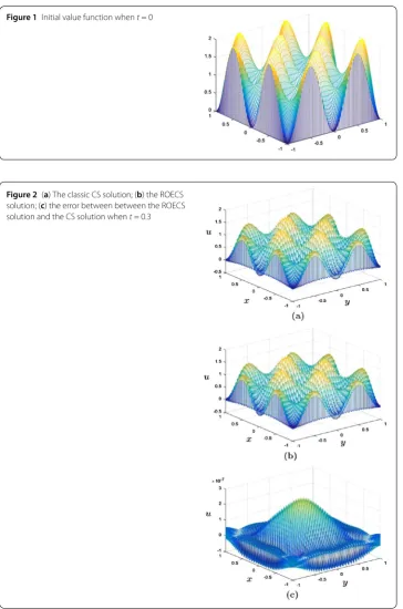
Example1 In the Sobolev equations, we takef(x,y,t) = 2(cos2πxcos2πy– 1)exp(–2t), u0(x,y) = 1 –cos2πxcos2πy(depicted in Fig.1),ϕ(x,y,t) =u0(x,y)exp(–2t), ε= 1/π2,
Figure 1Initial value function whent= 0
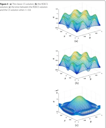
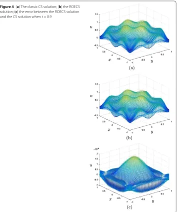
Figure 3(a) The classic CS solution; (b) the ROECS solution; (c) the error between the ROECS solution and the CS solution whent= 0.6
γ = 2/π2, the time stept= 0.01, and the number of nodes in two directionsN= 100,
q= 2.
We first compute the initialL= 20 coefficient vectorsUnN of the CS solutions of (11) at time nodestn(n= 1, 2, . . . , 20) to form the snapshot matrixP= (UN1,U2N, . . . ,U20N). Then
we find the eigenvalues λ1≥λ2≥ · · · ≥λ20≥0 and the associated eigenvectorsϕi(i=
1, 2, . . . ,r) ofPTPaccording to Step 2 in Sect.3.4. By computing we obtain that the error factor√λ7≤4×10⁻⁴. Thus, we only need to produce the POD basisΦ= (φ1,φ2, . . . ,φd)
by the formula φi =Pϕi/√λi (1≤i≤ d). Then, by the ROECS format, we find the
ROECS solutions atT = 0.3, 0.6, 0.9, respectively, depicted in (b) of Figs.2to4, respec-tively.
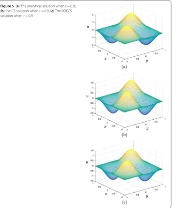
Figure 4(a) The classic CS solution; (b) the ROECS solution; (c) the error between the ROECS solution and the CS solution whent= 0.9
The comparison of (a) and (b) in Figs.2to4exhibits a quasi-identical similarity. In the computational process, the ROECS format at each time level only contains six unknowns, whereas the classic CS format has 10,201 unknowns. Therefore, the ROECS format can not only alleviate the calculation load and reduce the accumulation of round-off errors, but can also save CPU elapsed time and resources in the computational process. Photos (c) in Figs.2to4are, respectively, the errors between the ROECS solutions and the CS so-lutions whent= 0.3, 0.6, 0.9, which accord with the theoretical errors, because both errors areO(10–4).
Example2 To compare the CS and ROECS methods, we give another example, which also has an analytical solution for a 2D Sobolev equation. In the 2D Sobolev equation (1), we take ε= 1, γ = 10,f(x,y,t) = (12 +επ2 + 2γ π2)sinπxsinπyexp(t/2), u0(x,y) = sinπxsinπy,ϕ(x,y,t) = 0. Then this Sobolev equation has an exact solutionu(x,y,t) = sinπxsinπyexp(t/2).
First, we depict the exact solutionu(x,y,t) =et/2sinπxsinπyatT= 0.9 in (a) of Fig.5. Next, we take time stept= 0.01 and the number N= 100 of nodes in thexandy directions. By the classic CS format (4) we compute out the classic CS solution atT= 0.9, depicted in (b) of Fig.5.
Finally, to make a reasonable comparison, in solving the ROECS format, we adopt the same time step and number of nodes as in the classic CS format. We also compute the ini-tialL= 20 coefficient vectorsUnNof the CS solutions with the classic CS format (11) at time nodestn(n= 1, 2, . . . , 20) to form the snapshot matrixP= (UN1,U2N, . . . ,U20N). Then we find
the eigenvaluesλ1≥λ2≥ · · · ≥λ20≥0 and the associated eigenvectorsϕi(i= 1, 2, . . . ,r)
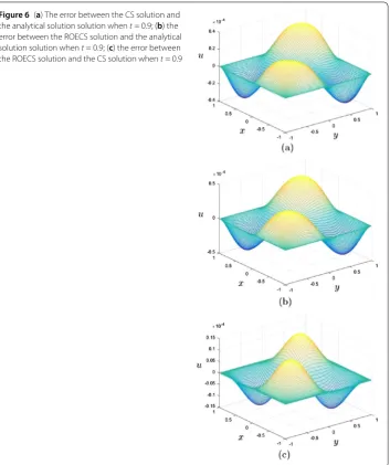
Figure 6(a) The error between the CS solution and the analytical solution solution whent= 0.9; (b) the error between the ROECS solution and the analytical solution solution whent= 0.9; (c) the error between the ROECS solution and the CS solution whent= 0.9
of PTP according to Step 2 in Sect. 3.4. By computing we obtain that the error factor
√
λ7≤2×10⁻⁴, so that it is only necessary to adopt the most main six POD bases Φ= (φ1,φ2, . . . ,φd) by the formulaφi=Pϕi/
√
λi(1≤i≤d) when solving the ROECS
for-mat. The obtaining ROECS solution atT= 0.9 is depicted in (c) of Fig.5.
Moreover, we depict the errors between the analytical solution and CS solution, the analytical solution and ROECS solution, and the CS solution and ROECS solution atT= 0.9 in photos (a), (b), and (c) of Fig.6, respectively.
for instance, it takes only about 260 s when computing the ROECS solution atT= 0.9, but takes 7033 s when computing the classic CS solution at the same time in the same Laptop (Microsoft Surface Book: Int Core i7 Processor, 16 GB RAM).
5 Conclusions and discussions
In this study, we have studied the reduced-order of the coefficient vectors of the solutions for the classic CS method of 2D Sobolev equations. We have established the ROECS for-mat in for-matrix form for 2D Sobolev equations via the POD technique, proven the existence, uniqueness, stability, and convergence of the ROECS solutions by the matrix means, and also given the flowchart for solving the ROECS format of 2D Sobolev equations. More-over, we have supplied two numerical examples to verify the correctness of the theoretical analysis to explain that the ROECS format is far superior to the classic CS format because the unknowns of the ROECS format are far fewer than those of the classic CS format, so that, compared to the classic CS format, the ROECS format can greatly lessen the compu-tational load, retard the round-off error accumulation, and save the CPU consuming time in the operational process.
Especially, the ROECS format for the 2D Sobolev equations is first presented in this paper and is a development and improvement over the existing reduced-order methods because the ROECS format has higher accuracy than other reduced-order methods, such as the reduced-order FE method, FVE method, and FD scheme. Both theory and method of this paper are new and completely different from the existing reduced-order methods. Although we restrict our ROECS method to Sobolev equations on rectangular domain Ω= [a,b]×[c,d], our technique can be extended to more general domains and applied in more complex engineering problems. Therefore, our technique has important applied prospect.
Acknowledgements
The authors are thankful to the honorable reviewers and editors for their valuable suggestions and comments, which improved the paper.
Funding
This research was supported by the National Science Foundation of China grant 11671106 and Qian Science Cooperation Platform Talent grant [2017]5726-41.
Availability of data and materials
The authors declare that all data and material in the paper are available and veritable.
Competing interests
The authors declare that they have no competing interests.
Authors’ contributions
Both authors contributed equally and significantly in writing this article. Both authors wrote, read, and approved the final manuscript.
Author details
1School of Control and Computer Engineering, North China Electric Power University, Beijing, China.2School of Mathematics and Physics, North China Electric Power University, Beijing, China.
Publisher’s Note
Springer Nature remains neutral with regard to jurisdictional claims in published maps and institutional affiliations.
Received: 11 October 2018 Accepted: 21 March 2019
References
2. Shi, D.M.: On the initial boundary value problem of nonlinear equation of the migration of the moisture in soil. Acta Math. Appl. Sin.13(1), 31–38 (1990)
3. Liu, Y., Li, H., He, S., Gao, W., Mu, S.: A new mixed scheme based on variation of constants for Sobolev equation with nonlinear convection term. Appl. Math. J. Chin. Univ.28(2), 158–172 (2013)
4. Shi, D.Y., Wang, H.H.: Nonconforming H1-Galerkin mixed FEM for Sobolev equations on anisotropic meshes. Acta Math. Appl. Sin.25(2), 335–344 (2009)
5. Guo, B.Y.: Some progress in spectral methods. Sci. China Math.56(12), 2411–2438 (2013) 6. Guo, B.Y.: Spectral Methods and Their Applications. World Scientific, Singapore (1998)
7. Zhou, Y.J., Luo, Z.D.: A Crank–Nicolson collocation spectral method for the two-dimensional telegraph equations. J. Inequal. Appl.2018, 137 (2018)
8. Shen, J., Tang, T.: Spectral and High-Order Methods with Applications. Science Press, Beijing (2006)
9. Luo, Z.D., Teng, F.: A reduced-order extrapolated finite difference iterative scheme based on POD method for 2D Sobolev equation. Appl. Math. Comput.329, 374–383 (2018)
10. Gao, F.Z., Qiu, J.X., Zhang, Q.: Local discontinuous Galerkin finite element method and error estimates for one class of Sobolev equation. J. Sci. Comput.41, 436–460 (2009)
11. Jiang, Z.W., Chen, H.Z.: Error estimates for mixed finite element methods for Sobolev equation. Northeast. Math. J.
17(3), 301–314 (2001)
12. Li, H., Luo, Z.D., An, J.: A fully discrete finite volume element formulation for Sobolev equation and numerical simulations. Math. Numer. Sin.34(2), 163–172 (2010)
13. Shi, D.Y., Wang, H.H., Guo, C.: Anisotropic rectangular nonconforming finite element analysis for Sobolev equations. Appl. Math. Mech.29(9), 1203–1214 (2008)
14. Luo, Z.D., Teng, F., Chen, J.: A POD-based reduced-order Crank–Nicolson finite volume element extrapolating algorithm for 2D Sobolev equations. Math. Comput. Simul.146, 118–133 (2018)
15. Lu, W.J., Zhang, F.Y.: Long-time behavior of completely discrete Fourier spectral method of solutions to Sobolev equations. J. Nat. Sci. Heilongjiang Univ.18(2), 5–8 (2001)
16. Jin, S.J., Luo, Z.D.: A collocation spectral method for the two-dimensional Sobolev equations. Bound. Value Probl.
2018, 53 (2018)
17. Cazemier, W., Verstappen, R.W.C.P., Veldman, A.E.P.: Proper orthogonal decomposition and low-dimensional models for driven cavity flows. Phys. Fluids10(7), 1685–1699 (1998)
18. Holmes, P., Lumley, J.L., Berkooz, G.: Turbulence, Coherent Structures, Dynamical Systems and Symmetry. Cambridge University Press, Cambridge (1996)
19. Ly, H.V., Tran, H.T.: Proper orthogonal decomposition for flow calculations and optimal control in a horizontal CVD reactor. Q. Appl. Math.60(4), 631–656 (1989)
20. Sirovich, L.: Turbulence and the dynamics of coherent structures: parts I–III. Q. Appl. Math.45(3), 561–590 (1987) 21. Fukunaga, K.: Introduction to Statistical Recognition. Academic Press, New York (1990)
22. Jolliffe, I.T.: Principal Component Analysis. Springer, Berlin (2002)
23. Selten, F.M.: Baroclinic empirical orthogonal functions as basis functions in an atmospheric model. J. Atmos. Sci.
54(16), 2099–2114 (1997)
24. Kunisch, K., Volkwein, S.: Galerkin proper orthogonal decomposition methods for parabolic problems. Numer. Math.
90(1), 117–148 (2001)
25. Kunisch, K., Volkwein, S.: Galerkin proper orthogonal decomposition methods for a general equation in fluid dynamischs. SIAM J. Numer. Anal.40(2), 492–515 (2002)
26. Luo, Z.D., Chen, J., Navon, I.M., Yang, X.Z.: Mixed finite element formulation and error estimates based on proper orthogonal decomposition for the non-stationary Navier–Stokes equations. SIAM J. Numer. Anal.47(1), 1–19 (2008) 27. Luo, Z.D., Li, H., Zhou, Y.J., Xie, Z.H.: A reduced finite element formulation based on POD method for two-dimensional
solute transport problems. J. Math. Anal. Appl.385(1), 371–383 (2012)
28. Cao, Y.H., Luo, Z.D.: A reduced-order extrapolating Crank–Nicolson finite difference scheme for the Riesz space fractional order equations with a nonlinear source function and delay. J. Nonlinear Sci. Appl.11, 672–682 (2018) 29. Luo, Z.D., Yang, X.Z., Zhou, Y.J.: A reduced finite difference scheme based on singular value decomposition and
proper orthogonal decomposition for Burgers equation. J. Comput. Appl. Math.229(1), 97–107 (2009)
30. Sun, P., Luo, Z.D., Zhou, Y.J.: Some reduced finite difference schemes based on a proper orthogonal decomposition technique for parabolic equations. Appl. Numer. Math.60(1–2), 154–164 (2010)
31. Luo, Z.D., Li, H., Zhou, Y.J., Huang, X.M.: A reduced FVE formulation based on POD method and error analysis for two-dimensional viscoelastic problem. J. Math. Anal. Appl.385(1), 310–321 (2012)
32. Luo, Z.D., Xie, Z.H., Shang, Y.Q., Chen, J.: A reduced finite volume element formulation and numerical simulations based on POD for parabolic problems. J. Comput. Appl. Math.235(8), 2098–2111 (2011)
33. Benner, P., Cohen, A., Ohlberger, M., Willcox, A.K.: Model Reduction and Approximation: Theory and Algorithm. Computational Science and Engineering. SIAM, Philadelphia (2017)
34. Hesthaven, J.S., Rozza, G., Stamm, B.: Certified Reduced Basis Methods for Parametrized Partial Differential Equations. Springer, Berlin (2016)
35. Quarteroni, A., Manzoni, A., Negri, F.: Reduced Basis Methods for Partial Differential Equations. Springer, Berlin (2016) 36. Luo, Z.D., Chen, G.: Proper Orthogonal Decomposition Methods for Partial Differential Equations. Mathematics in
Science and Engineering. Elsevier, Amsterdam (2018). https://www.elsevier.com/books/proper-orthogonal-decomposition-methods-for-partial-differential-equations/luo/978-0-12-816798-4
37. Luo, Z.D., Gao, J.Q.: A POD-based reduced-order finite difference time-domain extrapolating scheme for the 2D Maxwell equations in a lossy medium. J. Math. Anal. Appl.444, 433–451 (2016)
38. Luo, Z.D., Li, H.: A POD reduced-order SPDMFE extrapolating algorithm for hyperbolic equations. Acta Math. Sci. Ser. B Engl. Ed.34(3), 872–890 (2014)
39. Luo, Z.D., Li, H., Sun, P., Gao, J.Q.: A reduced-order finite difference extrapolation algorithm based on POD technique for the non-stationary Navier–Stokes equations. Appl. Math. Model.37(7), 5464–5473 (2013)
41. Luo, Z.D., Teng, F.: Reduced-order proper orthogonal decomposition extrapolating finite volume element format for two-dimensional hyperbolic equations. Appl. Math. Mech.38(2), 289–310 (2017)
42. An, J., Luo, Z.D., Li, H., Sun, P.: Reduced-order extrapolation spectral-finite difference scheme based on POD method and error estimation for three-dimensional parabolic equation. Front. Math. China10(5), 1025–1040 (2015) 43. Luo, Z.D., Jin, S.J.: A reduced-order extrapolation spectral-finite difference scheme based on the POD method for 2D
second-order hyperbolic equations. Math. Model. Anal.22(5), 569–586 (2017) 44. Adams, R.A.: Sobolev Spaces. Academic Press, New York (1975)
45. Zhang, W.S.: Finite Difference Methods for Partial Differential Equations in Science Computation. Higher Education Press, Beijing (2006) (in Chinese)