R E S E A R C H
Open Access
Fast two-phase image segmentation based
on diffusion equations and gray level sets
Boying Wu, Xiaoping Ji and Dazhi Zhang
**Correspondence:
Department of Mathematics, Harbin Institute of Technology, Harbin, 150001, China
Abstract
In this paper we propose a new scheme for image segmentation composed of two stages: in the first phase, we smooth the original image by some filters associated with noise types, such as Gaussian filters for Gaussian white noise and so on. Indeed, we propose a novel diffusion equations scheme derived from a non-convex functional for Gaussian noise removal in this paper. In the second phase, we apply a variational method for segmentation in the smoothed image domain obtained in the first phase, where we directly calculate the minimizer on the discrete gray level sets. In contrast to other image segmentation methods, there is no need for us to re-initialize parameters, which deduces the complexity of our algorithm toO(N) (Nis the number of pixels) and provides significant efficiency improvement when dealing with large-scale images. The obtained numerical results of segmentation on synthetic images and real world images both clearly outperform the main alternative methods especially for images contaminated by noise.
Keywords: two-phase segmentation; discrete gray level set; forward-backward diffusion; non-convex functional; Chan-Vese minimal variance
1 Introduction
Images are the proper -D projections of the -D world containing various objects. To re-construct the -D world perfectly, at least approximately, the first crucial step is to identify the regions in images that correspond to individual objects. This is the well-known prob-lem as image segmentation which has broad applications in a variety of important fields such as computer vision and medical image processing.
Image segmentation has been studied extensively in the past decades. A well-established class of methods consists of active contour models, which have been widely used in image segmentation with promising results. In general, these models apply variational meth-ods where they minimize some energy functionals depending on the features of the im-age. Classical ways to solve such problems are to solve the corresponding Euler-Lagrange equations. The existing active contour models can be roughly categorized into two classes: region-based models [–] and edges-based models [–]. A literature review of major active contour models can be found in [–].
Based on image gradient information, edges-based models drive one or more initial curve(s) to the boundaries of objects in the image. However, edges-based models are usu-ally sensitive to noise and weak edges information []. Instead of utilizing image gradient information, region-based models typically aim to identify each region of interest by us-ing a certain region descriptor, such as intensity, color, texture, to guide the motion of the
contour []. Therefore region-based models tend to rely on global information to steer contour evolution, which increase the chance to have better performance in the presence of image noise and weak object boundaries. In addition, region-based models are less sen-sitive to the initial contour locations than edge-based models. For instance, Chan and Vese [] developed an active contour without edge model to deal with image segmentation by using the level-set framework introduced by Osher and Sethian [], which is similar to the segmentation method independently proposed by Tsaiet al.[]. The active contour methods based on level-set framework have several following advantages. Firstly, they can deal with topological changes such as breaking and merging. Secondly, intrinsic geomet-ric elements such as the normal vector and the curvature can be easily interpreted with respect to the level-set function. Finally, this level-set framework can be extended and applied in any dimension.
However, these active contour methods based on level-set framework have some draw-backs. Firstly, most of these methods have initialization problems: different initial curves produce different segmentations because of the non-convexity of Chan-Vese models []. Secondly, these methods are usually implemented by solving corresponding evolution equations that suffer from severe numerical stability constrains which render them in-efficient. For instance, Chan-Vese models become severely inefficient due to the signed distance re-initialization procedure for stability reason. Recently, some researchers devel-oped fast algorithms [–] to the Chan-Vese image segmentation model to avoid these drawbacks above. In [–], the authors developed fast algorithms based on calculating the variational energy of the Chan-Vese model directly without the length term. In [], the authors proposed a fast method for image segmentation without solving the Euler-Lagrange equation of the underlying variational problem proposed by Chan and Vese, therefore they calculated the energy directly and checked if the energy is decreased when they change a point inside the level set to outside or vice versa.
2 Two-phase segmentation model
In this section, we show a two-stage scheme for implementation of the piecewise constant segmentation model. More precisely, the smoother version of the original image is first obtained by some smooth filter, and then, minimizing the Chan-Vese minimal variance criterion on the gray level sets, the image is divided into two subregions. Based on the idea above, we deal with the problem in two phases, respectively. Firstly, we propose a new denoising functional to obtain smoothing images. Secondly, we consider the continuous model of the new two-phase segmentation model based on gray level sets to propose the associated discrete model and then obtain a new algorithm.
2.1 The non-convex functional for Gaussian noise removal
In our two-phase algorithm, the second phase is fixed and can be easily performed and the new method depends in a large part on the smooth versionuof the original image. So it is better to use different edge-preserving denoising models for various types of noise.
According to conclusions in [], the non-convex functional may provide better or sharper edges than the convex functional does. In the smoothing phase of our method, the following edge-preserving denoising model is considered
min
E(u) =
α
|∇u|αdx+λ
|u–f|dx
, (.)
where <α< . Note that for <α< , the model is non-convex, so the edges will be pro-tected and even enhanced. However, the model above is an ill-posed problem. According to the proof given by Chipotet al.[], we have the following theorem.
Theorem . If f(x)is not a constant and f ∈L∞(),the function E(u)has no minimizer in W,()andinfu∈W,()E(u) = .
Proof We only prove the one-dimensional case= (a,b), and the same proof goes for N≥.
By density, we may always find a sequence of step functionsu˜nsuch that
|˜un| ≤ |f|L∞, lim
n→+∞|˜un–f|L()= .
In fact, we can find a partitiona=x<x<· · ·<xn=bsuch thatu˜nis the constantu˜n,ion
each interval (xi,xi),hn=maxi(xi–xi–) < withlimn→+∞hn= . Let us setσi=xi–xi–. Next, we define a sequence of continuous functionsunby
un(x) = ⎧ ⎨ ⎩
˜
un ifx∈[xi–,xi–σi/(–α)],
˜
un,i+–u˜n,i
σi/(–α) (x–xi) +u˜n,i+ ifx∈[xi–σ /(–α)
i ,xi].
Note that
|˜un–un|L()=
n
i=
xi
xi–σi/(–α)
(u˜n,i+–u˜n,i)
x–xi
σi/(–α) +
dx
≤ |f|
L∞()
n
i=
≤ |f|
L∞()h(+ α)/(–α)
n n i= σi = |f|
L∞()(b–a)h(+ α)/(–α)
n ,
and therefore,
lim
n→+∞|˜un–un|L()= .
Since
|un–f|L()≤ |˜un–un|L()+|˜un–f|L(),
and then taking the limit on both sides yields
lim
n→+∞|un–f|L()= .
Moreover,
α
b
a
|∇u|αdx=
α
n
i=
xi
xi–σi/(–α)
(u˜n,i+–u˜n,i)α
σiα/(–α) dx
≤
α
α|f|α
L∞()
n
i=
σi≤ α
α|f|α
L∞()hn n i= σi = α α|
f|αL∞()hn(b–a).
Thus
lim
n→+∞
α
b
a
|∇u|αdx= ,
and finally,
≤ inf
u∈W,()E(u)≤n→lim+∞E(un) = ,
i.e.,
inf
u∈W,()E(u) = .
Now, if there exists a minimizeru∈W,(), then necessarilyE(u) = , which implies
b
a
|u–f|dx= ⇔ u=f a.e.,
α
b
a
The first equality is possible only iff ∈W,(), and in this case the second equality implies f = , which is possible only iff is a constant. Therefore, excluding this trivial case,E(u)
has no minimizer inW,().
Remark . As we all know, if the regionis bounded, W,()⊂W,()⊂BV(),
then
inf
u∈W,()E(u)≥u∈Winf,()E(u)≥u∈infBV()E(u).
Note thatE(u)≥, and therefore
inf
u∈BV()E(u) = .
However, we cannot obtain any information about the minimizer ofE(u) inBV(). From the Euler-Lagrange equation for (.), we can obtain the following diffusion equa-tion:
∂u
∂t =div
|∇u|α–∇u–λ(u–f), (x,t)∈×T, (.)
u(x, ) =f, x∈, (.)
∂u
∂n
∂= , (x,t)∈∂×T. (.)
Remark .(Segmentation for various types of noisy image) There are lots of methods to obtain the smooth image in the first phase of the new method.
• If the type of noise is ‘salt and pepper’, for example, the AMF (adaptive median filter) can be selected;
• If the noise is ‘addition Gaussian noise’, for example, the Gaussian lower-pass filter, the new non-convex functional(.), the TV method (total variation model) [], the PM method (Perona-Malik model) [], and other anisotropic diffusion [] methods can be used to smooth the original image;
• If the noise is ‘multiplication noise’, for example, the SO method (Shi-Osher Model), which is an effective multiplicative noise removal model [], can be used to denoise the original image.
2.2 Chan-Vese minimal variance criterion based on gray level sets
First let us review the following Chan-Vese minimal variance criterion
F(c,c,φ) =
(u–c)H(φ)dx dy+
(u–c) –H(φ)dx dy. (.)
Assume that the smooth imageuis the solution from diffusion equations (.)-(.). Let
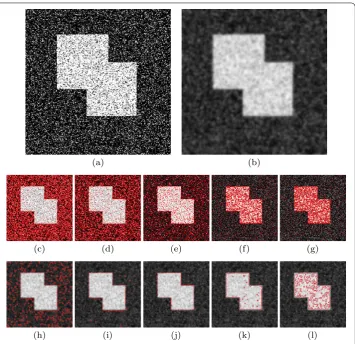
Figure 1 The level lines at different gray levels. (a)The noise image with Gaussian white noise of mean 0 and variance 0.2.(b)The smooth image by Gaussian low-pass filter withσ= 1.5.(c)-(g)The level lines of the noise image at the gray level 60, 80, 120, 180, and 200.(h)-(l)The level lines of the smooth image at the gray level 60, 80, 120, 180, and 200.
disorderly and irregular; while for the smooth image,∂χK is smooth and regular. These
basic facts are illustrated in Figure , where some∂χKare very close to the real edges of
the original image.
Hence, the level-set function can be replaced by the image gray functionuin the Chan-Vese minimal variance criterion [], and the new model is as follows:
F(K) =
(u–c)H(u–K)dx dy+
(u–c) –H(u–K)dx dy, (.)
where
c=
uH(u–K)dx
H(u–K)dx
, c=
u( –H(u–K))dx
( –H(u–K))dx
, (.)
and the Heaviside functionH
H(z) =
⎧ ⎨ ⎩
ifz≥,
Minimizing the function above, the best threshold is obtained, and then the image is seg-mented into two subregions{(x,y);u≥K}and{(x,y);u(x,y) <K}.
Notice that
F(K) =
udx–c
H(u–K)dx–c
–H(u–K)dx, (.)
c
H(u–K)dx+c
–H(u–K)dx=
f dx, (.)
forKm=minx∈u,
F(Km) =
(u–c)dx, c=u= ||
u dx,
and forKM=maxx∈u,
F(KM) =
(u–c)dx, c=u= ||
u dx.
Theorem . Assume f ∈L(), and then there exists the minimizerK∈[Km,KM]of F(K). Furthermore,if f is not a constant function,then the minimizer is the minimum point with F(K) = .
Proof Iff ∈L(),u∈C() andF(K)∈C[K
m,KM], there exists the minimizerK∗ ∈
[Km,KM] ofF(K). Noted thatg(α) =
(u–α)dxget the minimal atα=u, and then
(u–c)H(u–K)dx≤
(u–u)H(u–K)dx,
(u–c)
–H(u–K)dx≤
(u–u) –H(u–K)dx.
Hence
F(K)≤F(KM) =F(Km) forK∈[Km,KM],
which implies that the minimizer is the minimum point. By the Fermat theorem, we obtain that there existsK∈(Km,KM) such thatF(K) = .
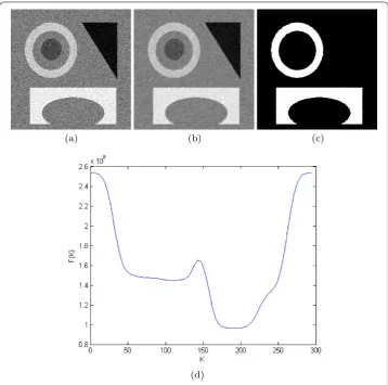
For any images we can always obtain the functionF(K). Figure (d) shows the function F(K) for the image in Figure (a). From the figure, we can see thatF(K) has the global minimizer and has several local minimizers.
Based on the new model (.), the two-phase algorithm is sketched below.
Algorithm .
. (Smoothing)By(.)-(.)obtain some appropriate smooth versionuof the noise imagef.
Figure 2 Segmentation results by Algorithm 2.1. (a)The noise image.(b)The smooth image by Gaussian low-pass filter withσ= 0.1.(c)The segmentation result (K= 169).(d)The functionF(K).
2.3 Discrete version of model (2.6)
Letui,j, for (i,j)∈D≡ {, . . . ,M} × {, . . . ,N}, be the gray level of a trueM-by-N image uat pixel location (i,j), and let [Km,KM] be the range of the smooth imageu,i.e.,Km≤
ui,j≤KM. LetD⊂DandD=D\D, and then the imageuis divided into two regions.
InsteadH(φ) byD, and ( –H(φ)) byD, respectively. Then minimizing the energy (.) is changed into minimize
F(c,c,D,D) =
(i,j)∈D
(ui,j–c)+
(i,j)∈D
(ui,j–c), (.)
with
c=
(i,j)∈Dui,j
|D| , c=
(i,j)∈Dui,j
|D| , (.)
It is noticed that since the selection of D andD is arbitrary, there are lots of pairs (D,D), so minimizing the energyFis difficult. Now, we introduce the following defini-tion, which contains a limited number of elements.
Definition .(Discrete gray level set) TheK-discrete gray level setDK, which is the set
of pixel location (i,j), is defined as follows
DK(i,j) :ui,j<K
,
whereui,jis the gray level of the imageuat pixel location (i,j).
For anyK∈[Km,KM], the imageuis divided into two subregions,i.e.,DK {(k,l) :uk,l<
K}andDK {(k,l) :uk,l≥K}. ThenDK =D\DK. LetA{(DK,DK),K∈[Km,KM]}, and
then the element numberNAof the setAisNA=KM–Km+ which is less than in
general. Then minimizing the energy (.) is changed into minimize
F(K) = (i,j)∈DK
(ui,j–c)+
(i,j)∈DK
(ui,j–c), for
DK,DK∈A (.)
with
c=
(i,j)∈DK ui,j |DK
|
, c=
(i,j)∈DK ui,j |DK
|
. (.)
Theorem .
min (D,D),D⊂D
F(c,c,D,D) = min (DK,DK)∈A
F(K). (.)
Proof It is clear that min(D,D),D⊂DF ≤ min(DK
,DK)∈AF. We only need to prove
min(D,D),D⊂DF≥min(DK,DK)∈AF.
From Theorem ., there exist two subdomainsD∗ andD∗such that
Fc∗,c∗,D∗,D∗= min
(D,D),D⊂DF(c,c,D,D).
Without loss of generality, assumec≤cand there exist (i,j)∈D∗and (i,j)∈D∗such thatui,j>ui,j. DenoteD=D∗– (i,j) + (i,j) andD=D∗– (i,j) + (i,j). Note that |D∗|=|D|,|D∗|=|D|,c∗>candc∗<c.
Having compared the energyF(c∗,c∗,D∗,D∗) andF(c,c,D,D), we get
Fc∗,c∗,D∗,D∗–Fc,c,D,D
=
(i,j)∈D∗
ui,j–c∗
+
(i,j)∈D∗
ui,j–c∗
–
(i,j)∈D
ui,j–c
–
(i,j)∈D
ui,j–c
=D∗c+c∗c–c∗+D∗c+c∗c–c∗
=c+c∗(ui,j–ui,j) +
c+c∗(ui,j–ui,j)
=c+c∗–c–c∗(ui,j–ui,j).
Sincec≤c, we have
c+c–c–c= c–
ui,j–ui,j |D| – c+
ui,j–ui,j |D| < .
So we get
F(c,c,D,D) >F
c,c,D,D.
SinceF(c,c,D,D) =min(D,D),D⊂DF(c,c,D,D), it is a contradiction. Therefore, for
any (i,j)∈D, (i,j)∈D, we haveui,j<ui,j. Hence there existsK∈[Km,KM] such that
ui,j<K≤ui,j,i.e., (D,D)∈A. We complete the proof of the theorem.
From (.) and (.), we can easily see that
F(c,c,D,D) =
(i,j)∈D
(ui,j–c)+
(i,j)∈D
(ui,j–c)
=
(i,j)∈D
ui,j–|D|c–|D|c. (.)
Hence we have the following.
Theorem . min(DK
,DK)∈AF(K)is equivalent to
max (DK,DK)∈A
E(K)DKc+DKc, (.)
where K∈[Km,KM],cand cis defined as(.).
Now, if the energy functionalEreaches a maximum, the best segmentation results are obtained,i.e., the subregionDK
and subregionDK. SinceK=Km,Km+, . . . ,KM, the energy
functionalE hasKM–Km+ cases, and then the maximum ofE is easily found. The
algorithm in the second phase is sketched below.
Algorithm . The method of maximizing the following functional E
. Sweep the imageuonce,record the number of all pixels at every gray level of the imageuwhich range fromKmtoKM.
. Calculate the energyE(K)by(.)forK∈[Km,KM],and find the maximizerK.
. The imageuis divided into two subregions,i.e.,DK ={(i,j) :u<K}and DK ={(i,j) :u≥K}.
Algorithm .
• (Smoothing)For the input noise imagef,use the Gaussian smooth filter or diffusion equations(.)-(.)to obtain the smooth imageu(if the input image is noiseless,this step is optional).
• (Minimal variance)Use Algorithm.to obtain the segmentation results for the smooth imageu.
3 Simulations
In this section, numerical examples on some synthetic and real world images are presented to illustrate the efficiency and effectiveness of our new two-phase scheme. The simulations are performed in Matlab Rb on a . GHz Pentium processor. For comparison pur-pose, the Chan-Vese method (CVM) [] is also tested. We utilize a locally one-dimensional (LOD) scheme adopted for CVM, which is an unconditional scheme [].
3.1 Configuration of smoothing filter
In the new algorithm, the first stage is smoothing the original image. The low-pass filtering is generally made by convolution with Gaussian of an increasing variance. Koenderink [] noticed that the convolution of signal with Gaussian at each scale was equivalent to the solution of the heat equation with the signal as initial datumf,i.e.,
∂u
∂t =u, (.)
u(x, ) =u. (.)
FFT (fast Fourier transform algorithm), the classical five-point explicit numerical schemes and the additive operator splitting (AOS) schemes can be used for the heat equation. In our experiment, we will use the Gaussian low-pass filter as one smoothing method in the first phase. For simplicity, we refer to the method as GLF-GLS (Gaussian low-pass filter-gray level set).
On the other hand, using the scheme in [], problems (.)-(.) can be discretized as
λ= , un+=
m
m
l=
I–mτAl
uk–un+λτf –un,
divn=un+–un/τ,
λn=
σMN(u–f)div
n,
ui,j=fi,j=f(ih,jh),
uni,=uni,, un,j=un,j, uIn,i=unI–,i, uni,J=uni,J–,
whereAl(un) = [ai,j(un)],
ai,j
un:=
⎧ ⎪ ⎪ ⎨ ⎪ ⎪ ⎩
Cn i+Cjn
h [j∈N(i)],
–n∈N(i)Cni+CNn
h (j=i),
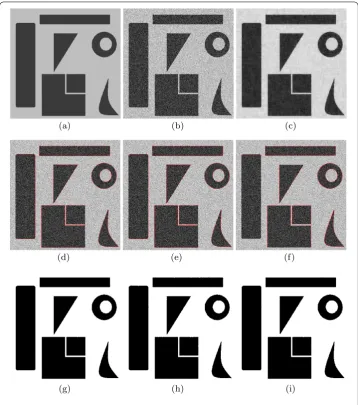
Figure 3 Segmentations for the noiseTest01image (size: 512×512).(a)The original image. (b)CorruptedTest01image with Gaussian noise (σ= 40).(c)SmoothedTest01image with the AOS scheme (τ= 70,α= 0.7, twice iterations).(d)Algorithm DE-GLS.(e)Algorithm GLF-GLS.(f)CVM.(g)-(i)The segmentation counter of Algorithm DE-GLS, Algorithm GLF-GLS and CVM, respectively.
and
Cin:=
ε+|∇uni,j|–α, where
∇uni,j=
p,q∈N(i) |un
p–unq|
h ,
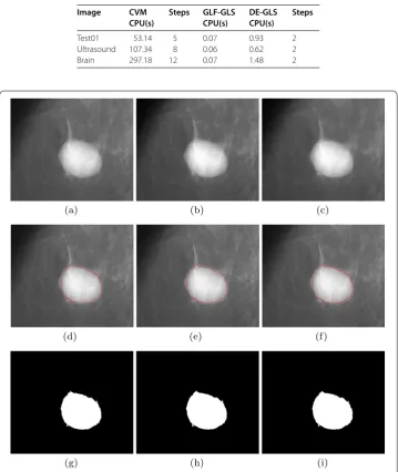
Table 1 Comparison of CPU time in seconds and iterate step
Image CVM
CPU(s)
Steps GLF-GLS
CPU(s)
DE-GLS CPU(s)
Steps
Test01 53.14 5 0.07 0.93 2
Ultrasound 107.34 8 0.06 0.62 2
Brain 297.18 12 0.07 1.48 2
Figure 4 Segmentations for the noiseultrasoundimage (size: 481×403). (a)The original image.(b)The smooth image by Gaussian low-pass filter withσ= 1.5.(c)Smoothedultrasoundimage with the AOS scheme (τ= 6,α= 0.9, twice iterations).(d)Algorithm DE-GLS.(e)Algorithm GLF-GLS.(f)CVM.(g)-(i)The
segmentation counter of Algorithm DE-GLS, Algorithm GLF-GLS and CVM, respectively.
PM scheme, a rather low price for gaining absolute stability []. Hence, in our numer-ical experiments, the AOS scheme is considered as the other smoothing method in the first phase. For simplicity, we refer to the two-phase method with the smoothing method as DE-GLS (diffusion equation-gray level set).
3.2 Segmentation performance
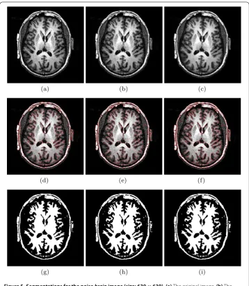
Figure 5 Segmentations for the noisebrainimage (size: 630×630). (a)The original image.(b)The smooth image by Gaussian low-pass filter withσ= 1.0.(c)Smoothedbrainimage with the AOS scheme (τ= 20,α= 0.6, twice iterations).(d)Algorithm DE-GLS.(e)Algorithm GLF-GLS.(f)CVM.(g)-(i)The segmentation counter of Algorithm DE-GLS, Algorithm GLF-GLS and CVM, respectively.
/ steps in Table ). However, re-initializing the level-set function costs a lot of CPU time (Table ). In the new method, GLF-GLS cost very little time (Table ) and for DE-GLS, it not only costs little time, but also has a very good segmentation result, especially for some singular information, such as corners and edges of the image.
In Figures and , we illustrate the results of GLF-GLS and DE-GLS about the realbrain andultrasoundimage. Few differences between the segmented images are observed, but our method works much faster than CVM (Table ).
3.3 Computational complexity
low-pass filter. In the second segmentation stage, our algorithm only sweeps the image once, so the complexity of the stage is no more thanO(N). In Table , we compare the CPU time needed for all three algorithms. Especially, we see that our algorithm GLF-GLS is about .-. seconds and is the fastest out of the three algorithms.
4 Summary
In this paper, we have proposed and implemented a novel image segmentation algorithm based on the Chan-Vese active contour model. The discrete gray level-set method is em-ployed in our numerical implementation. This algorithm works in two steps, we first smooth the noisy image by using the heat equation filter method, and then we utilize the new discrete gray level-set method to segment the region of the original image. The pro-posed new segmentation algorithm does not require the initialization of the level-set func-tions, which is a difficult problem in the Chan-Vese segmentation algorithm. Each step of the proposed new segmentation algorithm is simple and easily implemented. In the first step, there are a lot of algorithms to get the smoothing version of the original image, and in the second step, we only sweep the image once and calculate (.) at every gray level (in fact, only gray level sets) and find the optimal gray level. In Table , we show the CPU time of the Chan-Vese method and our proposed method. Obviously, our method is much more efficient than the Chan-Vese method.
Competing interests
The authors declare that they have no competing interests.
Authors’ contributions
XJ and BW carried out the proof of the main part of this article, DZ corrected the manuscript, and participated in its design and coordination. All authors have read and approved the final manuscript.
Acknowledgements
This work is partially supported by the National Science Foundation of China (11271100, 11301113, 71303067), China Postdoctoral Science Foundation funded project (Grant No. 2012M510933, Grant No. 2013M541400).
Received: 22 August 2013 Accepted: 5 December 2013 Published:09 Jan 2014
References
1. Mumford, D, Shah, J: Optimal approximation by piecewise smooth functions and associated variational problems. Commun. Pure Appl. Math.42, 577-685 (1989)
2. Chan, TF, Vese, LA: Active contours without edges. IEEE Trans. Image Process.10(2), 266-277 (2001) 3. Tsai, A, Yezzi, A, Willsky, AS: Curve evolution implementation of the Mumford-Shah functional for image
segmentation, denoising, interpolation, and magnification. IEEE Trans. Image Process.10(8), 1169-1186 (2001) 4. Gao, S, Bui, T: Image segmentation and selective smoothing by using Mumford-Shah model. IEEE Trans. Image
Process.14(10), 1537-1549 (2005)
5. Vese, L, Chan, TF: A multiphase level set framework for image segmentation using the Mumford and Shah model. Int. J. Comput. Vis.50(3), 271-293 (2002)
6. Chan, TF, Yezrielev Sandberg, B, Vese, LA: Active contours without edges for vector-valued images. J. Vis. Commun. Image Represent.2(11), 130-141 (2000)
7. Paragios, N, Deriche, R: Geodesic active regions and level set methods for supervised texture segmentation. Int. J. Comput. Vis.46(3), 223-247 (2002)
8. Kimmel, R: Fast edge integration. In: Level Set Methods and Their Applications in Computer Vision, Chapter 3. Springer, New York (2003)
9. Li, C, Huang, R, Ding, Z, Gatenby, C, Metaxas, D, Gore, J: A variational level set approach to segmentation and bias correction of medical images with intensity inhomogeneity. In: Proceedings of Medical Image Computing and Computer Aided Intervention (MICCAI). Part II. Lecture Notes in Computer Science, vol. 5242, pp. 1083-1091. Springer, Berlin (2008)
10. Kass, M, Witkin, A, Terzopoulos, D: Snakes: active contour models. Int. J. Comput. Vis.1(4), 321-331 (1987) 11. Caselles, V, Catte, F, Coll, T, Dibos, F: A geometric model for active contours. Numer. Math.66, 1-31 (1993) 12. Malladi, R, Sethian, JA, Vemuri, BC: Shape modeling with front propagation: a level set approach. IEEE Trans. Pattern
Anal. Mach. Intell.17(2), 158-175 (1995)
13. Xu, C, Prince, J: Generalized gradient vector flow external forces for active contours. Signal Process.71(2), 131-139 (1998)
15. Osher, S, Paragios, N: Geometric Level Set Methods in Imaging, Vision, and Graphics. Springer, New York (2003) 16. Jain, AK, Zhong, Y, Dubuisson-Jolly, M: Deformable template models: a review. Signal Process.71(2), 109-129 (1998) 17. Cremers, D, Rousson, M, Deriche, R: A review of statistical approaches to level set segmentation: integrating color,
texture, motion and shape. Int. J. Comput. Vis.72(2), 195-215 (2007)
18. Shi, Y, Karl, W: A fast level set method without solving pdes. In: Proceedings of ICASSP 2005. Philadelphia, PA, USA, March 2005, vol. II, pp. 97-100 (2005)
19. Song, B, Chan, T: A fast algorithm for level set based optimization. Tech. Rep. CAM02-68, UCLA Dept. Math. (2002) 20. Pan, Y, Birdwell, JD, Djouadi, SM: Efficient implementation of the Chan-Vese models without solving PDEs. In:
Proceedings of International Workshop on Multimedia Signal Processing (Victoria, BC, Canada, Oct. 03-06), pp. 350-353 (2006)
21. He, L, Osher, SJ: Solving the Chan-Vese model by a multiphase level set algorithm based on the topological derivative. In: Proceedings of the 1st International Conference on ScaleSpace Variational Methods in Computer Vision (2007)
22. Pan, Y, Birdwell, DJ, Seddik, DM: An efficient bottom-up image segmentation method based on region growing, region competition and the Mumford Shah functional. In: Proceedings of International Workshop on Multimedia Signal Processing (Victoria, BC, Canada, Oct. 03-06), pp. 344-348 (2006)
23. Wang, X, Huang, D, Xu, H: An efficient local Chan-Vese model for image segmentation. Pattern Recognit.43, 603-618 (2010)
24. Aubert, G, Kornprobst, P: Mathematical Problems in Image Processing: PDE’s and the Calculus of Variations. App. Mathem. Sciences, vol. 147. Springer, Berlin (2002)
25. Chipot, M, March, R, Rosati, M, Vergara Caffarelli, G: Analysis of a nonconvex problem related to signal selective smoothing. Math. Models Methods Appl. Sci.7(3), 313-328 (1997)
26. Rudin, L, Osher, S, Fatemi, E: Nonlinear total variation based noise removal algorithms. Physica D60, 259-268 (1992) 27. Perona, P, Malik, J: Scale-space and edge detection using anisotropic diffusion. IEEE Trans. Pattern Anal. Mach. Intell.
12(7), 629-639 (1990)
28. Weickert, J: Applications of nonlinear diffusion in image processing and computer vision. Acta Math. Univ. Comen.
70(1), 33-50 (2000)
29. Shi, J, Osher, S: A nonlinear inverse scale space method for a convex multiplicative noise model. SIAM J. Imaging Sci.
1(3), 294-321 (2008)
30. Koenderink, JJ: The structure of image. Biol. Cybern.50, 363-370 (1984)
31. Weickert, J, Romeny, B, Viergever, M: Efficient and reliable scheme for nonlinear diffusion filtering. IEEE Trans. Image Process.7(3), 398-410 (1998)
10.1186/1687-2770-2014-11
Cite this article as:Wu et al.:Fast two-phase image segmentation based on diffusion equations and gray level sets.