R E S E A R C H
Open Access
A first-order adjoint and a second-order
hybrid method for an energy output
least-squares elastography inverse problem
of identifying tumor location
Nathan D Cahill
1, Baasansuren Jadamba
1, Akhtar A Khan
1*, Miguel Sama
2and Brian C Winkler
1*Correspondence: [email protected] 1Center for Applied and
Computational Mathematics, School of Mathematical Sciences, Rochester Institute of Technology, 85 Lomb Memorial Drive, Rochester, NY 14623, USA
Full list of author information is available at the end of the article
Abstract
In this paper we investigate the elastography inverse problem of identifying cancerous tumors within the human body. From a mathematical standpoint, the elastography inverse problem consists of identifying the variable Lamé parameter
μ
in a system of linear elasticity where the underlying object exhibits nearly incompressible behavior. This problem is subsequently posed as an optimization problem using an energy output least-squares (EOLS) functional, but the nonlinearity that arises makes the computation of the EOLS functional’s derivatives challenging. We employ an adjoint method for the computation of the gradient, something shown to be an efficient method in recent studies, and also give a parallelizable hybrid method for the computation of the EOLS functional’s second derivative. Detailed discrete formulas and nontrivial computational examples are provided to show the feasibility of both the adjoint and hybrid approaches. Furthermore, all results are given in the framework of a general saddle point problem allowing easy adaptation to numerous other inverse problems.
MSC: 35R30; 65N30
Keywords: inverse problems; parameter identification; nearly incompressible elasticity; tumor identification; energy output least squares; output least squares; regularization; mixed finite element method; saddle point problems
1 Introduction
Consider the following system of partial differential equations describing the response of an isotropic elastic object to certain body forces and traction applied to its boundary:
–∇ ·σ=f in, (a)
σ= μ(u) +λdivuI, (b)
u=g on, (c)
σn=h on. (d)
Here the domainis a subset ofRorRand∂=∪is its boundary. In (a)-(d), the vector-valued functionu=u(x) represents the displacement of the elastic object,f is
the applied body force,nis the unit outward normal, and
(u) =
∇u+∇uT
is the linearized strain tensor. The resulting stress tensorσ in the stress-strain law (b) is obtained under the assumption that the elastic object is isotropic and the displacement is small enough so that a linear relationship holds. The Lamé parametersμandλquantify the elastic properties of the material. (In the following, for simplicity we setg= .)
In this work our objective is to investigate the elastography (also known as elasticity imaging) inverse problem of locating cancerous tumors within the human body. This in-verse problem consists of identifying the variable parameterμin (a)-(d) from a mea-surement of the displacement fieldu. Conversely, the direct problem for (a)-(d) is to find the displacementuwhen functionh, the variable coefficientsμandλ, and the body forcef are all known. The underlying idea is that differences in molecular makeup as well as microscopic and macroscopic structure result in significant differences in the stiffness of living soft tissue (see []). Moreover, changes in tissue stiffness generally correlate with changes in pathological state, with many cancers appearing as hard nodules within the surrounding softer tissue. In a clinical setting, measurements of displacement in human tissue can be obtained using ultrasound and this can then serve as data in the context of the elastography inverse problem. By solving this inverse problem and recoveringμ, tumor locations can be identified using the marked differences in elastic properties between the healthy and unhealthy tissue. Additionally, we note that in the elastography inverse prob-lem the human body is treated as a nearly incompressible object where the parameterλis significantly large and hence only the parameterμis sought.
Although numerous authors have contributed to using the elasticity properties of soft tissue as a tool to differentiate between normal and cancerous tissue, Raghavan and Yagle [] were among the first authors to realize that this study can be best done in an inverse problem framework using measured strains and the equations of equilibrium to recover elasticity (cf.(a)-(d)). Since then, many studies have been devoted to investigating var-ious aspects of the elastography inverse problem and the interested reader is referred to [–] and the cited reference therein. Additionally, a detailed account of the recent devel-opments in elastography inverse problem can be found in the survey article by Doyley []. See also [–] and the cited references therein for more details.
One of the main technical challenges in the study of this inverse problem stems from the fact that the human body is treated as a nearly incompressible object. That is, the elasticity modulusλis significantly large (and particularlyλμ), rendering classical finite element methods ineffective due to the so-called locking effect. In the literature, several approaches have been proposed to overcome the locking effect, and in this work we employ the mixed finite elements strategy.
In the following, we provide the necessary details for the transformation of system (a)-(d) into a saddle point problem to which the mixed finite element approach can be ap-plied.
We begin by recalling that the dot product of two tensorsAandBcan be denoted by
A·B. That is, for × tensorsAandB, we have
Given a sufficiently smooth domain⊂R, theL-norm of a tensor-valued function
A=A(x) is given by
AL=AL()=
A·A=
A+A+A+A.
On the other hand, for a vector-valued functionu(x) = (u(x),u(x))T, theL-norm is given by
uL=uL()=
u+u,
whereas theH-norm by
uH=uH()=uL+∇uL.
In the following discussion, for the sake of simplicity, in (a)-(d) we setg= . For this case, the space of test functions, denoted byV, is given by
V=¯v∈H()×H() :v¯= on
.
By using Green’s identity and boundary conditions (c) and (d), we obtain the following weak form of elasticity system (a)-(d): Findu¯∈Vsuch that
μ(u¯)·(v¯) +
λ(divu¯)(divv¯) =
fv¯+
¯
vh for everyv¯∈V. ()
The mixed finite elements strategy, which, in the present context, consists of introducing a pressure termp∈Q=L(), is as follows:
divu¯=p
λ. ()
Asλ→ ∞, () yields the incompressibility limit
divu¯= .
The weak formulation of () reads
(divu¯)q–
λpq= for everyq∈Q. ()
By using relation (), the weak form () can be expressed as follows: Findu¯∈Vsuch that
μ(u¯)·(v¯) +
p(divv¯) =
fv¯+
¯
vh for everyv¯∈V, ()
Therefore, the problem of findingu¯∈V, satisfying (), has now been converted into the saddle point problem of finding (u¯,p)∈V×Qsuch that
μ(u¯)·(v¯) +
p(divv¯) =
fv¯+
¯
vh for everyv¯∈V, (a)
(divu¯)q–
λpq= for everyq∈Q, (b)
whereQ=L() andV={¯v∈H()×H() :v¯= on }.
For the saddle point formulation, the Babuška-Brezzi condition provides guidance in the choice of finite element spaces necessary for a stable numerical approximation (see []). The primary objective of this work is to develop an efficient computational framework for the elastography inverse problem. For this we employ an adjoint approach for the derivative computation of a recently proposed energy output least-squares (EOLS) func-tional []. We recall that Oberai et al.[] used the adjoint approach to compute ef-ficiently the gradient of the output least-squares functional. Inspired by Tortorelli and Michaleris [], we also devise a hybrid method for an efficient computation of the second-order derivative of the EOLS functional. In this direction, we would also like to draw at-tention to an interesting paper by Cioacaa, Alexea, and Sandua [] where a second-order adjoint method is studied. All the results and formulas given are for a general saddle point problem and hence can easily be adapted to a wide range of inverse problems for varia-tional problems (see []). In the derivation of the adjoint formulas, we do not include the regularization functional while considering the EOLS functional. However, we use a smooth regularizer for the identification of a smooth parameter and a BV regularizer for the identification of discontinuous coefficients.
2 Optimization approach for inverse problems in saddle point problems
LetVandQbe real Hilbert spaces, letBbe a real Banach space, and letAbe a nonempty, closed, and convex subset ofB. HereBis the coefficient/parameter space andAis the set of all admissible coefficients. Let a:B×V ×V →Rbe a trilinear map which we assume to be symmetric with respect to the second and third arguments. That is, for every
∈Band for allu¯,v¯∈V, we havea(,u¯,v¯) =a(,v¯,u¯). Letb:V×Q→Rbe a bilinear form, letc:Q×Q→Rbe a symmetric bilinear form, and letm:V→Rbe a linear and continuous map. We assume that there are positive constantsκ,κ,ς,ς, andκsuch that the following inequalities hold:
a(,v¯,v¯)≥κ¯v for everyv¯∈V, for every∈A, (a)
a(,u¯,v¯)≤κ¯u¯v for everyu¯,¯v∈V, for every∈A, (b)
c(q,q)≥ςq for everyq∈Q, (c)
c(p,q)≤ςpq for everyp,q∈Q, (d) b(v¯,q)≤κ¯vq for every¯v∈V, for everyq∈Q. (e)
required to be compactly embedded in the solution space (see [–]). In our discrete examples, we have used linear elements to approximate the imposed box-constraints.
We consider the following saddle point problem: Given∈A, find (u¯,p)∈V×Qsuch that
a(,u¯,¯v) +b(¯v,p) =m(¯v) for everyv¯∈V, (a)
b(u¯,q) –c(p,q) = for everyq∈Q. (b)
Given all the data, the direct problem in this setting is to find (u¯,p). However, our focus is on the inverse problem of finding a parameter ∈Athat makes (a)-(b) true for a measurement (z¯,zˆ) of (u¯,p).
Evidently, saddle point problem (a)-(b) connected to the elastography inverse prob-lem of identifying a variable parameterμin the system of incompressible linear elasticity can be deduced by setting:
a(μ,u¯,v¯) =
μ(u¯)·(¯v), (a)
b(u¯,q) =
(divu¯)q, (b)
c(p,q) =
λpq, (c)
m(v¯) =
fv¯+
¯
vh. (d)
A common approach to solve inverse problems of parameter identification in PDEs is to minimize the output least-squares functional, which, in the present context, can be defined by
JOLS() =
u() –z
V=
u¯() –z¯
V+
p() –zˆ
Q, ()
whereV =V×Q,z= (z¯,zˆ)∈V is the measured data, andu() = (u¯(),p())∈V is the solution of (a)-(b) corresponding to.
The output least-squares solution to the inverse problem of identifyingis the one that solves the following optimization problem: Find¯∈Asuch that
JOLS(¯)≤JOLS() for every∈A.
Recently, in [], the following objective functional was proposed to solve the inverse problem of identifying the variable parameter∈Ain saddle point problem (a)-(b):
J() = a
,u¯() –z¯,u¯() –z¯+ c
p() –ˆz,p() –zˆ, ()
Clearly, to solve an optimization problem with the above objective functional, we need to compute its derivative which, in turn, requires us to compute the derivative of the solution map. It is well known that one of the most challenging aspects in the study of inverse problems is in finding an efficient computation of the derivative of the solution map. We will now develop an adjoint method for the computation of the first derivative of the EOLS functional and then a new hybrid method for the computation of the functional’s second derivative.
For every∈A, the map→S() = (u¯(),p()) is well defined and single-valued. The following result for the differentiability ofS, which was announced in [] without a proof, will be needed.
Theorem . For eachin the interior of A,u=u() = (u¯(),p())is infinitely differentiable at.
. Givenu,the first derivativeδu= (δu¯,δp) = (Du¯()δ,Dp()δ)is the unique solution of the saddle point problem:
a(,δu¯,v¯) +b(¯v,δp) = –a(δ,u¯,v¯) for everyv¯∈V, (a)
b(δu¯,q) –c(δp,q) = for everyq∈Q. (b)
. The second-order derivative
δu=δu¯,δp=Du¯()(δ,δ),Dp()(δ,δ)
is the unique solution of the saddle point problem
a,δu¯,v¯+bv¯,δp= –aδ,Du¯()δ,v¯
–aδ,Du¯()δ,v¯ for everyv¯∈V, (a)
bδu¯,q–cδp,q= for everyq∈Q. (b)
Proof We define a mapG:A×V→V∗×Q∗byG(, (u¯,p)) = (a(,u¯)+b(p)–m,b(u¯)–c(p)), whereV∗andQ∗are the duals ofVandQ, anda(,u¯),b(p), andc(p) are the associated dual elements given by the Riesz theorem. Then saddle point problem (a)-(b) is equivalent to the following implicit equation:
G(,u) = (V∗, Q∗). ()
The differentiability ofu=u() follows from the implicit function theorem. In fact, the mapGis infinitely differentiable and the partial derivative with respect to variableu= (u¯,p) is given by
DuG
, (u¯,p)(δu¯,δp)≡a(,δu¯) +b(δp),b(δu¯) –c(δp) for everyδu¯∈V.
By [, Proposition ], the mapDuG(, (u¯,p)) :A×V→V∗×Q∗is an isomorphism.
We now compute the first and second derivatives of the coefficient-to-solution map. By using equation (a), for anyˆ∈Aand for any sufficiently smallt∈R+, we have
a+tˆ,u¯(+tˆ),v¯+bv¯,p(+tˆ)=m(v¯),
a,u¯(),v¯+bv¯,p()=m(v¯),
and by manipulating the terms in these two equations, we obtain
a
+tˆ,u¯(+tˆ) –u¯()
t ,v¯
+aˆ,u¯(),¯v+b
¯
v,p(+tˆ) –p()
t
= ,
which, by passing the above equation to the limit whent→+, yields (a)
a,Du¯()(ˆ),v¯+bv¯,Dp()(ˆ)= –aˆ,u¯(),v¯.
Analogously, using equation (b), for anyˆ∈Aand for every sufficiently smallt∈R+, we have
bu(+tˆ),q–cp(+tˆ),q= ,
bu(),q–cp(),q= ,
and by manipulating the above two equations, we obtain
b
u(+tˆ) –u()
t ,q
–c
p(+tˆ) –p()
t ,q
= ,
which, by passing the above equation to limitt→+, gives
bDu¯()(ˆ),q–cDp()(ˆ),q= ,
which is (b). Consequently, (a) and (b) characterize the first derivative.
The same arguments can be used to compute the form of the second derivative. From (a), for anyˆ,ˆ∈Aand for any sufficiently smallt∈R+, we have
a+tˆ,Du¯(+tˆ)(ˆ),v¯
+b¯v,Dp(+tˆ)(ˆ)
= –aˆ,u¯(+tˆ),v¯
,
a,Du¯()(ˆ),v¯+bv¯,Dp()(ˆ)= –aˆ,u¯(),v¯, and by rearranging the above set of equations, we obtain
aˆ,Du¯(+tˆ)(ˆ),v¯
+a
,Du¯(+tˆ)(ˆ) –Du¯()(ˆ)
t ,v¯
+b
¯
v,Dp(+tˆ)(ˆ) –Dp()(ˆ)
t
= –a
ˆ
,u¯(+tˆ) –u¯()
t ,v¯
Since the solution mapu=u() is twice Fréchet differentiable, by passing to the limit
t→+, we get
aˆ,Du¯()(ˆ),v¯+a,Du¯(ˆ,ˆ),v¯+bv¯,Dp(ˆ,ˆ)
= –aˆ,Du¯()(ˆ),v¯, ()
which, after a rearrangement of terms, yields (a)
a,Du¯(ˆ,ˆ),v¯
+bv¯,Dp(ˆ,ˆ)
= –aˆ,Du¯()(ˆ),v¯
–aˆ,Du¯()(ˆ),v¯
.
From (b), for anyˆ,ˆ∈Aand any sufficiently smallt∈R+, we have
bDu¯(+ˆ)(ˆ),q–cDp(+ˆ)(ˆ),q= ,
bDu¯()(ˆ),q–cDp()(ˆ),q= ,
and by rearranging the above two equations, we get
b
Du¯(+tˆ)(ˆ) –Du¯()(ˆ)
t ,q
–c
Dp(+ˆ)(ˆ) –Dp()(ˆ)
t ,q
= .
By passing to limitt→+, we finally deduce
bDu¯(ˆ,ˆ),q–cDp(ˆ,ˆ),q= ,
which in conjunction with (b) forms the corresponding saddle point whose unique so-lution characterizes the second derivativeDu(ˆ,ˆ) = (Du¯(ˆ,ˆ),Dp(ˆ,ˆ)).
3 An adjoint and a hybrid method for the energy output least squares
The developed adjoint method for the EOLS functional,
J() =
a(,u¯–z¯,u¯–z¯) +
c(p–zˆ,p–zˆ),
is based on the key observation that the underlying saddle point problem can equivalently be posed as a variational equation of findingu= (u¯,p)∈V=V×Qsuch that
T(,u,v) =m(v¯) for everyv= (v¯,q)∈V, () where
T(,u,v) =a(,u¯,v¯) +b(v¯,p) +b(u¯,q) –c(p,q). () By a direct computation, we have
DT(,u,v)()(δ) =a(δ,u¯,¯v) +a(,δu¯,¯v) +b(v¯,δp) +b(δu¯,q) –c(δp,q)
We define
J(,v) =J() +T(,u,v) –m(¯v) for everyv∈V,
and, by using (), notice that
J(a,v) =J(a) for everyv∈V.
Therefore, for any ‘test function’v= (v¯,q)∈V, we have
DJ()(δ) =DJ(,v)(δ) for everyδ∈A, ()
whereDstands for the partial derivative with respect to.
The key idea behind the adjoint method is to choose a particularvto avoid the compu-tation ofδu. By a direct computation and taking into account (), we obtain
DJ(,v)(δ) =
a(δ,u¯–z¯,u¯–¯z) +a(,δu¯,u¯–z¯) +c(δp,p–ˆz)
+a(δ,u¯,v¯) +T(,δu,v). () Now, letw=w() be the unique solution of the saddle point problem
a(,w¯,v¯) +b(v¯,pw) = –a(,u¯–¯z,v¯) –b(¯v,p–zˆ) for everyv¯∈V, (a)
b(w¯,q) –c(pw,q) = for everyq∈Q, (b)
which exists, by standard arguments, since the above problem is just (a)-(b) withm(·) = –a(,u¯,·) –b(·,p).
By settingv=win (), we obtain
DJ(,w)(δ) =
a(δ,u¯–z¯,u¯–z¯) +a(,δu¯,u¯–z¯) +c(δp,p–zˆ) +a(δ,u¯,w¯) +T(,δu,w)
=
a(δ,u¯–z¯,u¯–z¯) +a(,δu¯,u¯–z¯) +c(δp,p–zˆ) +a(δ,u¯,w¯) –a(,u¯–z¯,δu¯) –b(δu¯,p–ˆz) =
a(δ,u¯–z¯,u¯–z¯) +a(δ,u¯,w¯) +a(,δu¯,u¯) +c(δp,p) –b(δu¯,p–zˆ) +a(δ,u¯,w¯) –a(,δu¯,u¯–¯z)
=
a(δ,u¯–z¯,u¯–z¯) +a(δ,u¯,w¯) +c(δp,p–zˆ) –b(δu¯,p–zˆ),
where we have used the symmetry of the trilinear formT,a(,·,·), and (a)-(b). Since
c(δp,p–zˆ) =b(δu¯,p–zˆ), we obtain
DJ(,w)(δ) =
Therefore, using (), we have
DJ()(δ) =
a(δ,u¯–¯z,u¯–z¯) +a(δ,u¯,w¯). () Summarizing, we have the following scheme to compute the derivative DJ() given
a∈A:
. Computeuby().
. Computewby(a)-(b). . ComputeDJ()by().
Let us now develop the hybrid method for the computation of the second-order deriva-tive. In the hybrid method proposed below, the derivativeδuis computed directly while the computation of the second derivativeδuis avoided by using an adjoint method. We will follow the same general scheme that was used above, but here we will use derivative formula (a)-(b).
Letδ∈Abe a fixed direction. Then, for anyv= (¯v,q)∈V, we define
H(,v) =DJ()(δ) +a,Du¯()(δ),¯v+bv¯,Dp()(δ) +bDu¯()(δ),q–cDp()(δ),q+a(δ,u¯,v¯) =
a(δ,u¯–z¯,u¯–z¯) +a
,Du¯()(δ),u¯–z¯
+cDp()(δ),p–zˆ
+a,Du¯()(δ),v¯
+bv¯,Dp()(δ)
+bDu¯()(δ),q–cDp()(δ),q+a(δ,u¯,v¯). By the construction ofH, for everyv∈V, we have
∂H
∂(,v)(δ) =D
J()(δ
,δ) for everyδ∈A. () By a simple calculation, we have
∂H
∂(,v)(δ) =a
δ,Du¯()(δ),u¯–¯z+aδ,Du¯()(δ),u¯–z¯
+a,Du¯()(δ,δ),u¯–z¯
+a,Du¯()(δ),Du¯()(δ)
+cDp()(δ,δ),p–zˆ+cDp()(δ),Dp()(δ) +aδ,Du¯()(δ),v¯+a,Du¯()(δ,δ),v¯
+bv¯,Dp()(δ,δ)
+bDu¯()(δ,δ),q
–cDp()(δ,δ),q
+aδ,Du¯()(δ),v¯
. ()
Letw() = (w¯(),pw()) be the unique solution of the saddle point problem (cf.(a)-(b)):
a(,w¯,v¯) +b(v¯,pw) =a(,v¯,z¯–u¯) +b(v¯,zˆ–p) for everyv¯∈V, (a)
By settingv=win (), we have
∂H
∂(,w)(δ) =a
δ,Du¯()(δ),u¯–z¯+aδ,Du¯()(δ),u¯–z¯
+a,Du¯()(δ,δ),u¯–¯z+a,Du¯()(δ),Du¯()(δ) +cDp()(δ,δ),p–ˆz+cDp()(δ),Dp()(δ) +aδ,Du¯()(δ),w¯+a,Du¯()(δ,δ),w¯
+bw¯,Dp()(δ,δ)+bDu¯()(δ,δ),q
–cDp()(δ,δ),q+aδ,Du¯()(δ),w¯
=aδ,Du¯()(δ),u¯–z¯+aδ,Du¯()(δ),u¯–z¯
+a,Du¯()(δ),Du¯()(δ)+cDp()(δ),Dp()(δ)
+a,Du¯()(δ,δ),u¯–z¯+cDp()(δ,δ),p–zˆ
+aδ,Du¯()(δ),w¯+a,Du¯()(δ,δ),w¯
+bw¯,Dp()(δ,δ)+bDu¯()(δ,δ),q
–cDp()(δ,δ),q+aδ,Du¯()(δ),w¯
=aδ,Du¯()(δ),u¯–z¯+aδ,Du¯()(δ),u¯–z¯
+a,Du¯()(δ),Du¯()(δ)+cDp()(δ),Dp()(δ)
+aδ,Du¯()(δ),w¯+aδ,Du¯()(δ),w¯
+cDp()(δ,δ),p–ˆz+bDu¯()(δ,δ),ˆz–p. Recall that by derivative formula (a)-(b), we have
cDp()(δ,δ),p–zˆ=bDp()(δ,δ),p–zˆ, which implies
∂H
∂(,w)(δ) =a
δ,Du¯()(δ),u¯–z¯+aδ,Du¯()(δ),u¯–z¯
+a,Du¯()(δ),Du¯()(δ)
+cDp()(δ),Dp()(δ)
+aδ,Du¯()(δ),w¯
+aδ,Du¯()(δ),w¯
.
Consequently, from (), we get
DJ()(δ,δ) =aδ,Du¯()(δ),u¯–z¯+aδ,Du¯()(δ),u¯–z¯
+a,Du¯()(δ),Du¯()(δ)+cDp()(δ),Dp()(δ) +aδ,Du¯()(δ),w¯+aδ,Du¯()(δ),w¯
and, in particular,
Summarizing, we propose the following scheme to compute the derivativeDJ()(δ,δ) given∈A,δ∈A.
. Computeu() = (u¯(),p)by(). . Computeδu= (δu¯,δp)by(a)-(b). . Computew() = (w¯(),q())by(a)-(b). . ComputeDJ()(δ,δ)by().
4 Discretization formulas for the adjoint and the hybrid method
In this section, we collect discrete formulae for saddle point problem (a)-(b) and the associated inverse problem. We begin, therefore, with a triangulationTh on,Lh is the
space of all piecewise continuous polynomials of degreedrelative toTh,Uhis the space
of all piecewise continuous polynomials of degreedurelative toTh, andQhis the space of
all piecewise continuous polynomials of degreedqrelative toTh.
In order to represent the discrete saddle point problem in a computable form, we pro-ceed as follows. We represent bases forLh,Uh, andQhby{ϕ,ϕ, . . . ,ϕm},{ψ,ψ, . . . ,ψn},
and{χ,χ, . . . ,χk}, respectively. The spaceLhis then isomorphic toRmand for any∈Lh,
we defineL∈Rm byL
i =(xi) fori= , , . . . ,m, where the nodal basis{ϕ,ϕ, . . . ,ϕm}
corresponds to the nodes{x,x, . . . ,xm}. Conversely, eachL∈Rm corresponds to∈Lh
defined by=mi=Liϕi. Similarly,u∈Uh will correspond toU∈Rn, whereU¯i=u(yi),
i= , , . . . ,n, andu=ni=U¯iψi, wherey,y, . . . ,ynare the nodes of the mesh definingUh.
Finally,q∈Qhwill correspond toQ∈Rk, whereQi=q(zi),i= , , . . . ,k, andq=ki=Qiχi,
wherez,z, . . . ,zkare the nodes of the mesh definingQh. (The spacesAh,Uh, andQhare
defined relative to the same elements, but the nodes will be different ifd=du=dq.)
Recall that the discrete saddle point problem seeks, for eachh, the unique (u¯h,ph)∈
Vh×Qhwith
a(h,u¯h,v¯) +b(v¯,ph) =m(v¯) for everyv¯∈Uh, (a)
b(u¯h,q) –c(ph,q) = for everyq∈Qh. (b)
We defineS:Rm→Rn+kto be the finite element solution operator that assigns to each
coefficienth∈Ahthe unique approximate solutionuh= (u¯h,ph)∈Uh×Qh. ThenS(L) =
U, whereUis defined by
K(L)U=F, ()
and where the stiffness matrixK(L)∈R(n+k)×(n+k)and the load vectorF∈Rn+kare given
by
K(L) =
K(L) BT B –C
with
K(L)i,j=a(,ψj,ψi), i,j= , , . . . ,n,
Ci,j=c(χj,χi), i,j= , , . . . ,k,
Fi=m(ψi), i= , , . . . ,n,
Fj= , j=n+ ,n+ , . . . ,n+k.
For future reference, it will be useful to note that
K(L)ij=TijkLk,
where the summation convention is used andTis the tensor defined by
Tijk=a(ϕk,ψi,ψj) for everyi,j= , . . . ,n,k= , . . . ,m.
Let us now compute the discrete analogue of energy least-squares objective functional. By using the above notations, the discrete form of
J(L) =
a(,u¯–z¯,u¯–¯z) +
c(p–zˆ,p–zˆ) is given by
J(L) =
¯
U(L) –Z¯TK(L)U¯(L) –Z¯+
P(L) –ZTCP(L) –Z.
In order to get an operative expression for the gradient, we need to consider the so-called adjoint stiffness matrixAdefined by the following condition:
K(L)V¯ =A(V¯)L for everyL∈Rm, for everyV¯ ∈Rn. ()
4.1 Computation of the gradient by using the adjoint method
Using the above notation, we have the following discrete adjoint method for the compu-tation of gradient ofJ(·).
. We computeU=UP¯((LL))by solving the linear system
K(L) BT
B –C
¯
U(L)
P(L)
=
F
. ()
. We computeW=PW¯(L)
W(L)
by solving the linear system
K(L) BT
B –C
¯
W(L)
PW(L)
=
–K(L)(U¯ –Z¯) –BT(P–P)
. ()
. The gradient∇J(L)can be calculated by using the adjoint stiffness matrix. From
(), we have
DJ()(δ) =
a direct discretization gives the following:
∇J(L)(δL) = (U¯ –Z¯)
TK(δL)(U¯ –Z¯) +U¯TK(δL)W¯
= U¯
TA(U¯ –Z¯)δL+U¯TAW¯(L)δL,
and therefore the gradient∇J(L)is given by
∇J(L) = (U¯ –Z¯)
TA(U¯ –Z¯) +U¯TAW¯ (L). ()
4.2 Computation of the Hessian by using a hybrid method Recall that we have established the following:
DJ()(δ,δ) = a(δ,δu¯,u¯–z¯) +a(,δu¯,δu¯) +c(δp,δp) + a(δ,δu¯,w¯). () By the standard discretization scheme, we have
. a(δL,δU¯,U¯ –Z¯) =δLT∇ ¯UTK(δL)(U¯ –Z¯) =δLT∇ ¯UTA(U¯ –Z¯)δL,
. a(L,δU¯,δU¯) =δLT∇ ¯UTK(L)∇ ¯UδL=δLT∇ ¯UTK(L)∇ ¯UδL,
. c(δP,δP) =δLT∇PTC∇PδL,
. a(δ,δu¯,w¯) =δLT∇ ¯UTK(δL)W¯ =δLT∇ ¯UTA(W¯)δL.
Consequently, we have the following explicit formula for the Hessian:
∇J(L) = T∇ ¯UTA(U¯ –Z¯) +∇ ¯UTK(L)∇ ¯U+∇PTC∇P+ ∇ ¯UTA(W¯). ()
Summarizing, we have the following scheme for the computation of the second deriva-tive of the EOLS:
. ComputeU= (U¯,P)by solving linear system(). . ComputeW= (W¯,P)by solving linear system(). . Compute∇U= (∇ ¯U,∇P)by solvingmlinear systems. . Compute∇J(L)by using formula().
We note that to compute the Hessian using the hybrid method requires the solution of
m+ linear systems.
5 Numerical experiments
We consider here two representative examples of elastography inverse problems for the recovery of a variableμon a two-dimensional isotropic domain= (, )×(, ) with boundary∂=∪. In the first example, a smooth coefficient is recovered using both the adjoint and hybrid gradient calculation methods. For the second example, we examine the recovery of a discontinuous coefficient using the adjoint method.
All examples are solved on a × quadrangular mesh with , quadrangles and , total degrees of freedom. Example uses a smooth Tikhonov-type regulariza-tion method, whereas the discontinuities in Example necessitate the use of a BV-regularization scheme (see [] for a more thorough discussion of BV-regularization).
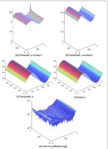
5.1 Example 1
Figure 1 Example 1 using adjoint method/1st-order algorithm (13 iterations).
boundaries have Neumann conditionh(x,y). The functions defining the coefficient, load, and boundary conditions are as follows:
μ(x,y) = . +
sin(πx), f(x,y) =
. +x
. +y
,
g(x,y) =
x y
on, h(x,y) =
+ x + y
Figure 2 Example 1 using hybrid method/2nd-order algorithm (9 iterations).
For this example, the underlying optimization problem was solved using both a first-order Newton-CG-Trust Region algorithm as well as a second-first-order quasi-Newton method, using the adjoint and hybrid gradient calculations outlined in the preceding sec-tions, respectively. Comparatively, the hybrid method converges faster to the solution in only algorithm iterations compared to iterations for the adjoint method when both are started from the same initial point and under the same stopping criteria (∇J< –). This can be seen qualitatively in Figures and through the comparison of the computed
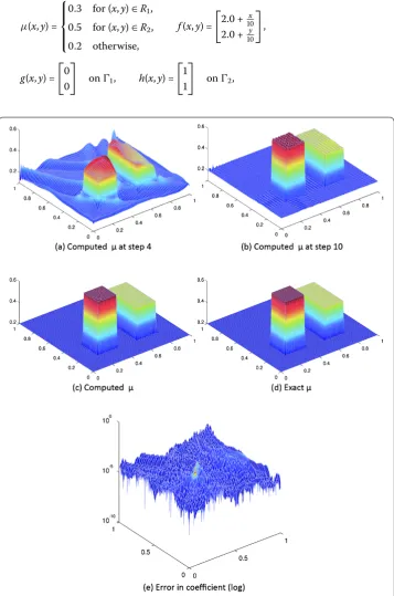
5.2 Example 2
For the discontinuous example, the top of the region is taken asand fixed with (con-stant) Dirichlet conditiong(x,y). The remaining edges of the region are taken aswith Neumann conditionh(x,y). The functions defining the coefficient, load, and boundary conditions are as follows:
μ(x,y) = ⎧ ⎪ ⎪ ⎨ ⎪ ⎪ ⎩
. for (x,y)∈R, . for (x,y)∈R, . otherwise,
f(x,y) =
. +x . +y
,
g(x,y) =
on, h(x,y) =
on,
whereR={(x,y) : .≤x≤., .≤y≤.}andR={(x,y) : .≤x≤., .≤y≤ .}.
6 Concluding remarks
In this work we have presented a detailed application of the adjoint method for efficiently computing the gradient of the energy output least-squares functional as well as a hybrid method for calculating the functional’s second derivative. We have also provided two nu-merical examples of elastography inverse problems to demonstrate the overall feasibility of implementation and establish the relative effectiveness of these methods when coupled with the appropriate first-order and second-order optimization algorithms. See Figure . One issue not addressed in depth was the comparative performance of these methods, measured both against existing schemes and against one other. In short, we note that the hybrid method requires the solution ofm+ linear systems withmscaling along with the size of the mesh. However, themsystems remain entirely independent, allowing for the parallelization of parts of the computation and thus granting significant performance gains and potential advantages over other strategies. In a future work, we look to extend our study here into just such a thorough analysis and carefully consider the performance of the adjoint and hybrid derivative computation methods.
Competing interests
The authors declare that they have no competing interests.
Authors’ contributions
This research was carried out during Prof. Miguel Sama’s visit at RIT and all the work was done at that time in a collaborative manner. All authors read and approved the final manuscript.
Author details
1Center for Applied and Computational Mathematics, School of Mathematical Sciences, Rochester Institute of
Technology, 85 Lomb Memorial Drive, Rochester, NY 14623, USA.2Departamento de Matemática Aplicada, Universidad
Nacional de Educación a Distancia, Calle Juan del Rosal, 12, Madrid, 28040, Spain.
Acknowledgements
The work of AA Khan is supported by RIT’s COS D-RIG Acceleration Research Funding Program 2012-2013 and a grant from the Simons Foundation (#210443 to Akhtar Khan). The work of M Sama is partially supported by Ministerio de Ciencia (Spain), project (MTM2012-30942).
Received: 14 August 2013 Accepted: 5 November 2013 Published:02 Dec 2013 References
1. Doyley, MM: Model-based elastography: a survey of approaches to the inverse elasticity problem. Phys. Med. Biol.57, R35 (2012). doi:10.1088/0031-9155/57/3/R35
2. Raghavan, KR, Yagle, AE: Forward and inverse problems in elasticity imaging of soft tissues. IEEE Trans. Nucl. Sci.41, 1639-1648 (1994)
3. Aguilo, MA, Aquino, W, Brigham, JC, Fatemi, M: An inverse problem approach for elasticity imaging through vibroacoustics. IEEE Trans. Med. Imaging29, 1012-1021 (2010)
4. Ammari, H, Garapon, P, Jouve, F: Separation of scales in elasticity imaging: a numerical study. J. Comput. Math.28, 354-370 (2010)
5. Arnold, A, Reichling, S, Bruhns, O, Mosler, J: Efficient computation of the elastography inverse problem by combining variational mesh adaption and clustering technique. Phys. Med. Biol.55, 2035-2056 (2010)
6. Beretta, E, Bonnetier, E, Francini, E, Mazzucato, A: Small volume asymptotics for anisotropic elastic inclusions. Inverse Probl. Imaging6, 1-23 (2012)
7. Ji, L, McLaughlin, J: Recovery of Lamé parameterμin biological tissues. Inverse Probl.20, 1-24 (2004)
8. Kallel, F, Bertrand, M: Tissue elasticity reconstruction using linear perturbation method. IEEE Trans. Med. Imaging15, 299-313 (1996)
9. Barbone, PE, Bamber, JC: Quantitative elasticity imaging: what can and cannot be inferred from strain images. Phys. Med. Biol.47, 2147-2164 (2002)
10. Barbone, PE, Gokhale, NH: Elastic modulus imaging: on the uniqueness and nonuniqueness of the elastography inverse problem in two dimensions. Inverse Probl.20, 283-296 (2004)
12. Chan, TF, Tai, XC: Identification of discontinuous coefficients in elliptic problems using total variation regularization. SIAM J. Sci. Comput.25, 881-904 (2003)
13. Gockenbach, MS, Khan, AA: Identification of Lamé parameters in linear elasticity: a fixed point approach. J. Ind. Manag. Optim.1, 487-497 (2005)
14. Gockenbach, MS, Jadamba, B, Khan, AA: Numerical estimation of discontinuous coefficients by the method of equation error. Int. J. Math. Comput. Sci.1, 343-359 (2006)
15. Gockenbach, MS, Jadamba, B, Khan, AA: Equation error approach for elliptic inverse problems with an application to the identification of Lamé parameters. Inverse Probl. Sci. Eng.16, 349-367 (2008)
16. Harrigan, T, Konofagou, EE: Estimation of material elastic moduli in elastography: a local method, and an investigation of Poisson ratio sensitivity. J. Biomech.37, 1215-1221 (2004)
17. Jadamba, B, Khan, AA, Raciti, F: On the inverse problem of identifying Lamé coefficients in linear elasticity. Comput. Math. Appl.56, 431-443 (2008)
18. Jadamba, B, Khan, AA, Sama, M: Inverse problems of parameter identification in partial differential equations. In: Mathematics in Science and Technology, pp. 228-258. World Scientific, Hackensack (2011)
19. Konofagou, E, Harrigan, T, Ophir, J, Krouskop, T: Poroelastography: estimation and imaging of the poroelastic properties of tissues. In: IEEE Proceedings of the Symposium in Ultrasonics, Ferroelectrics and Frequency Control, Lake Tahoe, NV, pp. 1627-1630 (1999)
20. McLaughlin, J, Yoon, JR: Unique identifiability of elastic parameters from time-dependent interior displacement measurement. Inverse Probl.20, 25-45 (2004)
21. Mehrabian, H, Campbell, G, Samani, A: A constrained reconstruction technique of hyperelasticity parameters for breast cancer assessment. Phys. Med. Biol.53, 7489-7508 (2012)
22. Brezzi, F, Fortin, M: Mixed and Hybrid Finite Element Methods. Springer, New York (1991)
23. Doyley, MM, Jadamba, B, Khan, AA, Sama, M, Winkler, B: A new energy inversion for parameter identification in saddle point problems with an application to the elasticity imaging inverse problem of predicting tumor location (2013, submitted)
24. Oberai, AA, Gokhale, NH, Feijóo, GR: Solution of inverse problems in elasticity imaging using the adjoint method. Inverse Probl.19, 297-313 (2003)
25. Tortorelli, DA, Michaleris, P: Design sensitivity analysis: overview and review. Inverse Probl. Eng.1, 71-105 (1994) 26. Cioacaa, A, Alexea, M, Sandua, A: Second-order adjoints for solving PDE-constrained optimization problems. Optim.
Methods Softw.27, 625-653 (2012)
27. Goeleven, D, Motreanu, D: Variational and Hemivariational Inequalities - Theory, Methods and Applications, vol. 2. Springer, Berlin (2003)
28. Bush, N, Jadamba, B, Khan, AA, Raciti, F: Identification of a parameter in fourth-order partial differential equations by an equation error approach (2014, to appear)
29. Crossen, E, Gockenbach, MS, Jadamba, B, Khan, AA, Winkler, B: An equation error approach for the elasticity imaging inverse problem for predicting tumor location. Comput. Math. Appl. (2013, to appear)
30. Gockenbach, MS, Khan, AA: An abstract framework for elliptic inverse problems. Part 1: an output least-squares approach. Math. Mech. Solids12, 259-276 (2007)
31. Gockenbach, MS, Khan, AA: An abstract framework for elliptic inverse problems. Part 2: an augmented Lagrangian approach. Math. Mech. Solids14, 517-539 (2009)
10.1186/1687-2770-2013-263