R E S E A R C H
Open Access
A spectral relaxation method for thermal
dispersion and radiation effects in a nanofluid
flow
Peri K Kameswaran, Precious Sibanda
*and Sandile S Motsa
*Correspondence:
sibandap@ukzn.ac.za
School of Mathematical Sciences, University of KwaZulu-Natal, Private Bag X01 Scottsville,
Pietermaritzburg, 3209, South Africa
Abstract
In this study we use a new spectral relaxation method to investigate heat transfer in a nanofluid flow over an unsteady stretching sheet with thermal dispersion and radiation. Three water-based nanofluids containing copper oxide CuO, aluminium oxide Al2O3and titanium dioxide TiO2nanoparticles are considered in this study. The
transformed governing system of nonlinear differential equations was solved numerically using the spectral relaxation method that has been proposed for the solution of nonlinear boundary layer equations. Results were obtained for the skin friction coefficient, the local Nusselt number as well as the velocity, temperature and nanoparticle fraction profiles for some values of the governing physical and fluid parameters. Validation of the results was achieved by comparison with limiting cases from previous studies in the literature. We show that the proposed technique is an efficient numerical algorithm with assured convergence that serves as an alternative to common numerical methods for solving nonlinear boundary value problems. We show that the convergence rate of the spectral relaxation method is significantly improved by using the method in conjunction with the successive over-relaxation method.
Keywords: spectral relaxation method; heat transfer; stretching sheet; nanofluids
1 Introduction
In recent years flow and heat transfer over a stretching surface has been extensively inves-tigated due to its importance in industrial and engineering applications such as in the heat treatment of materials manufactured in extrusion processes and the casting of materials. Controlled cooling of stretching sheets is needed to assure quality products. Fiber tech-nology, wire drawing, the manufacture of plastic and rubber sheets and polymer extrusion are some of the important processes that take place subject to stretching and heat transfer. The quality of the final product depends to a great extent on the heat controlling factors, and the knowledge of radiative heat transfer in the system can perhaps lead to a desired product with a sought characteristic.
The development of a boundary layer over a stretching sheet was first studied by Crane [], who found an exact solution for the flow field. This problem was then extended by Gupta and Gupta [] to a permeable surface. The flow problem due to a linearly stretch-ing sheet belongs to a class of exact solutions of the Navier-Stokes equations. Since the pioneering work of Sakiadis [], various aspects of the stretching problem involving
tonian and non-Newtonian fluids have been extensively studied by several authors (see Cortell [], Hayat and Sajid [], Liao [], Xu []).
The study of radiation effects has important applications in engineering. Thermal radi-ation effect plays a significant role in controlling heat transfer process in polymer process-ing industry. Many studies have been reported on flow and heat transfer over a stretched surface in the presence of radiation (see El-Aziz [, ], Raptis [], Mahmoud []). El-Aziz [] studied the radiation effect on the flow and heat transfer over an unsteady stretching sheet. He found that the heat transfer rate increases with increasing radiation and un-steadiness parameters and the Prandtl number. The effect of the radiation parameter on the heat transfer rate was found to be more noticeable at larger values of the unsteadiness parameter and the Prandtl number. In addition to radiation, it is important to consider the thermal dispersion effect on boundary layer flow since this has a direct impact on the heat transfer rate. Several studies on hydrodynamic dispersion have been reported in the literature. The double-dispersion phenomenon in a Darcian, free convection boundary layer adjacent to a vertical wall, using multi-scale analysis arguments, was investigated by Telles and Trevisan [].
In recent years tremendous effort has been given to the study of nanofluids. The word nanofluid coined by Choi [] describes a liquid suspension containing ultra fine parti-cles (diameter less than nm). Experimental studies (e.g., Masudaet al.[], Daset al. [], Xuan and Li []) showed that even with a small volumetric fraction of nanoparticles (usually less than %), the thermal conductivity of the base liquid is enhanced by -% with a remarkable improvement in the convective heat transfer coefficient. The litera-ture on nanofluids was reviewed by Trisaksri and Wongwises [], Wang and Mujumdar [] among several others. Nanofluids thus provide an alternative to many common fluids for advanced thermal applications in micro and nano-heat transfer applications. Thermo-physical properties of nanofluids such as thermal conductivity, diffusivity and viscosity were studied by Kanget al.[], Velagapudiet al.[], Rudyaket al.[]. Hadyet al.[] studied the radiation effect on the viscous flow of a nanofluid and heat transfer over a nonlinearly stretching sheet. They observed that the increase in the thermal radiation pa-rameter and the nonlinear stretching sheet papa-rameter yields a decrease in the nanofluid temperature leading to an increase in the heat transfer rate. The boundary layer flow of a nanofluid with radiation was studied by Olanrewajuet al.[]. They observed that ra-diation has a significant influence on both the thermal boundary layer thickness and the nanoparticle volume fraction profiles.
Recently, Mahdy [] studied the effects of unsteady mixed convection boundary layer flow and heat transfer of nanofluids due to a stretching sheet. He found that the heat trans-fer rate at the surface increased with the mixed convection parameter and the solid volume fraction of nanoparticles. Moreover, the skin friction increased with the mixed convection parameter and decreased with the unsteadiness parameter and the nanoparticle volume fraction. Narayana and Sibanda [] studied the effects of laminar flow of a nanoliquid film over an unsteady stretching sheet. They found that the unsteadiness parameter has the effect of thickening the momentum boundary layer while thinning the thermal bound-ary layer for Cu-water and AlO-water nanoliquids. Kameswaranet al.[] studied the
de-creased with an increase in the nanoparticle volume fraction, while the opposite was true in the case of temperature and concentration profiles.
The objective of this study is to analyze the effects of fluid and physical parameters such as thermal dispersion, nanoparticle volume fraction and radiation parameters on the flow and heat transfer characteristics of three different water based nanofluids containing cop-per oxide CuO, aluminium oxide AlO and titanium dioxide TiO nanoparticles. The
momentum and energy equations are coupled and nonlinear. By using suitable similar-ity variables, we convert these equations into coupled ordinary differential equations and solve them numerically via a novel iteration scheme called the spectral relaxation method (SRM) (see Motsa and Makukula [], Mosta []). The SRM is an iterative algorithm for the solution of nonlinear boundary layer problems which are characterized by flow prop-erties that decay exponentially to constant levels far from the boundary surface. The key features of the method are the decoupling of the governing nonlinear systems into a se-quence of smaller sub-systems which are then discretized using spectral collocation meth-ods. The method is very efficient in solving boundary layer equations of the type under investigation in this study. In cases where the SRM convergence is slow, it is demonstrated that successive over-relaxation can be used to accelerate convergence and improve the ac-curacy of the method. The current results were validated by comparison with published results in the literature and results obtained using the Matlabbvp4croutine. We further show that substantial improvement in the convergence rate of the SRM may be realized by using this method in conjunction with the successive over relaxation method.
2 Mathematical formulation
Transient unsteady-state flow and heat transfer (t> 0)
This study is concerned with the laminar boundary layer flow of an incompressible nanofluid over a stretching sheet. The origin of the system is located at the slit from which the sheet is drawn, withxandydenoting coordinates along and normal to the sheet. The fluid is a water-based nanofluid containing either alumina, copper-oxide or titanium-oxide nanoparticles. The base fluid and the nanoparticles are in thermal equilibrium and no slip occurs between them. The sheet is stretched with velocity
Uw(x,t) = bx –αt
alongx-axis, wherebandα are positive constants with dimensions (time)–andαt< . The surface temperature distribution
Tw(x,t) =T∞+T
bxr νf
( –αt)–m
varies both along the sheet and with time whereTis a reference temperature,T∞is the
ambient temperature andνf is the kinematic viscosity of the fluid. Under these assump-tions, the boundary layer equations governing the flow, heat and concentration fields can be written in a dimensional form (see Tiwari and Das []) as follows:
∂u ∂x +
∂v
∂u ∂t +u
∂u ∂x+v
∂u ∂y=
μnf ρnf
∂u
∂y, ()
∂T ∂t +u
∂T ∂x +v
∂T ∂y =αnf
∂T ∂y –
(ρCp)nf
∂qr ∂y +
∂ ∂y
αy ∂T
∂y
. ()
The initial conditions are:
u(x, ) =u(x), v(x, ) = , T(x, ) =Tw(x). ()
The appropriate boundary conditions for equations ()-() have the form:
u(x,t) =Uw(x,t), v(x,t) = , T(x,t) =Tw(x,t) aty= ,
u(x,t)→, T(x,t)→T∞ asy→ ∞,
()
whereu,vare the velocity components in thexandydirections, respectively, T is the fluid temperature,Cpis the specific heat at constant pressure,randmare constants, the
expression for the effective thermal diffusivity taken asαy=αm+γdu,αm is the molec-ular thermal diffusivity,γdurepresent thermal diffusivity,γ is the mechanical thermal dispersion coefficient anddis the pore diameter.
Following Rosseland’s approximation,Tis expressed as a linear function of the
tem-peratureT≡T
∞T– T∞ and the radiative heat fluxqris modeled as ∂qr
∂y = – σ∗T∞
k∗ ∂T
∂y, ()
whereσ∗is the Stefan-Boltzman constant andk∗is the mean absorption coefficient. The effective dynamic viscosity of the nanofluid was given by Brinkman as
μnf = μf
( –φ)., ()
whereφ is the solid volume fraction of spherical nanoparticles. The effective density of each nanofluid is given as
ρnf = ( –φ)ρf +φρs. ()
The thermal diffusivity of the nanofluid is
αnf = knf (ρCp)nf
, ()
where the heat capacitance of the nanofluid is given by
(ρCp)nf = ( –φ)(ρCp)f+φ(ρCp)s. ()
The thermal conductivity of the nanofluids is approximated by the Maxwell-Garnett (MG) model (Maxwell-Garnett [] and Guerinet al.[]):
knf =kf
ks+ kf– φ(kf–ks) ks+ kf+φ(kf –ks)
The subscriptsnf,f andsrepresent the thermophysical properties of the nanofluid, base fluid and nanoparticles, respectively. The continuity equation () is satisfied by introducing a stream functionψ(x,y,t), where
u=∂ψ
∂y and v= – ∂ψ
∂x, ()
with
ψ(x,y,t) =
νfb –αt
xf(η) and η=
b νf( –αt)
y, ()
wheref(η) is the dimensionless stream function. The velocity components are then given by
u=
bx –αt
f(η) and v= –
νfb –αt
f(η). ()
The temperature is represented as
T=T∞+ (Tw–T∞)g(η), ()
whereg(η) is the dimensionless temperature. On using equations ()-(), equations (), () and () transform into the following two-point boundary value problem:
f+φ
ff–f–S
η f
+f= , ()
g
+Df+kR φ
knf kf
+Dfg+Pr
fg–rfg–S
η g
+mg= , ()
f() = , f() = , f(∞)→, ()
g() = , g(∞)→, ()
where
kR= + NR
. ()
The non-dimensional constants in equations () and () are the unsteadiness parame-terS, the thermal dispersion parameterD, the radiation parameterNR and the Prandtl numberPr. They are respectively defined as
S=α
b, D=
γdUw αm
, NR=
knfk∗ σ∗T
∞
, Pr=νf(ρCp)f kf
, ()
where
φ= ( –φ).
–φ+φ
ρs ρf
and φ= –φ+φ
(ρCp)s (ρCp)f
. ()
Table 1 Thermophysical properties of water and nanoparticles, Oztop and Abu-Nada [33]
Properties→ ρ(kg/m3) C
p(J/kgK) k(W/mK)
Pure water 997.1 4,179 0.613
CuO 3,620 531.8 76.5
Al2O3 3,970 765 40
TiO2 4,250 686.2 8.9538
3 Skin friction and heat transfer coefficients
In addition to velocity and temperature, the quantities of engineering interest in heat transport problems are the skin friction coefficientCf and the local Nusselt numberNux. These parameters respectively characterize the surface drag and wall heat transfer rate. The shear stress at the wall is given by
τw= –μnf
∂u ∂y y= = –
( –φ).ρfν
f
b –αt
xf(). ()
The skin friction coefficient is defined as
Cf= τw ρfUw
, ()
and using equation () in equation (), we obtain
Cf( –φ).Re
x = –f(). ()
The heat transfer rate at the surface is given by
qw= –knf
∂T ∂y
y=
= –knf(Tw–T∞)
b νf( –αt)
g(). ()
The Nusselt number is defined as
Nux= x kf
qw
Tw–T∞. ()
Using equation () in equation (), we obtain the dimensionless wall heat transfer rate as Nux Re x kf knf
= –g(), ()
whereRexis the local Reynolds number defined byRex=xUw/νf.
4 Initial steady state flow and heat transfer (t≤0)
In the case of steady state solution,i.e.,S→, equations () and () along with boundary conditions () and () are replaced by
f+φ
g
+Df+kR φ
knf kf
+Dfg+Prfg–rfg
= , ()
f() = , f() = , f(∞)→, ()
g() = , g(∞)→. ()
The momentum boundary layer equation is partially decoupled from the energy equa-tion. The solution is obtained by looking for an exponential function of the formf(η) = e–sη that satisfies both the differential equation and governing boundary conditions over
the interval [,η], and the exact solution to () and () is
f(η) = –e
–sη
s , ()
wheresis a parameter associated with the nanoparticle volume fraction. This satisfies the equation
s=φ. ()
We note that from equation () we obtainf() = –s. In the case of a clear fluid, we have s= and solution () reduces to Crane’s solution for a stretching sheet problem given by
f(η) = –e–η withf() = –.
Here we presented the solution of a heat transfer equation in the absence of thermal dis-persion as a particular case. Equation () is replaced by
g–Pr
kf knf
φ
kR
rfg–fg
= . ()
Introducing a new variable
ξ= –Pr se
–sη
, ()
equation () and thermal boundary conditions () take the form:
ξgξ ξ+
–λ Pr∗+ξ
gξ+λrg= , ()
g –Pr∗= , g –→, ()
whereλ= (
kf
knf)
φ kR andPr
∗=Pr/sis the modified Prandtl number.
The solution of equation () is obtained in terms of confluent hypergeometric functions in the following form:
g(ξ) =CξαM[α–r,α+ ,λξ], ()
where
M[a,b,z] =
∞
r=
is Kummer’s function. Making use of boundary conditions () and rewriting the solution in terms of the variableη, we get
g(η) =e
–sηαM[α–r
,α+ , –αe–sη]
M[α–r,α+ , –α]
. ()
The surface heat transfer rate has the exact value
g() =(
α–r
α+)M[α–r+ ,α+ , –α] –SαM[α–r,α+ , –α]
M[α–r,α+ , –α]
, ()
where
α=λPr∗.
5 The spectral relaxation method
In this section we give a brief description of the spectral relaxation method (SRM) that is employed to solve equations ()-(); see also Motsa and Makukula []. The SRM is pro-posed for the solution of similarity boundary layer problems with exponentially decaying profiles. For self-similar boundary layer problems, the SRM algorithm may be summarized as follows:
. Reduce the order of the momentum equation forf(η)by introducing the transformationf(η) =p(η)and express the original equation in terms ofp(η). . Assuming thatf(η)is known from a previous iteration (denoted byfr), construct an
iteration scheme forp(η)by assuming that only linear terms inp(η)are to be evaluated at the current iteration level (denoted bypr+) and all other terms (linear
and nonlinear) are assumed to be known from the previous iteration. In addition, nonlinear terms inpare evaluated at the previous iteration.
. The iteration schemes for the other governing dependent variables are developed in a similar manner but now using the updated solutions of the variables determined in the previous equation.
The strategy described above is analogous to the Gauss-Seidel idea of decoupling linear al-gebraic system of equations. Using this algorithm leads to a sequence of linear differential equations with variable coefficients which can easily be solved using standard numerical techniques for solving linear differential equations. In this study we discretize the differen-tial equations using Chebyshev spectral collocation methods (see, for example, [, ]). Spectral methods are preferred here because of their remarkably high accuracy and ease of implementation in discretizing and the subsequent solution of variable-coefficient lin-ear differential equations with smooth solutions over simple domains. In the context of the SRM iteration scheme described above, equations ()-() become
pr++φfrpr+–φS
pr++
η p
r+
=φpr, ()
fr+=pr+, fr+() = , ()
gr++Dgr+pr++
knf kf
+
NR
φ
gr+
+Dpr+gr++Pr
fr+gr+–rpr+gr+–S
mgr++
η g
r+
subject to boundary conditions
pr+() = , pr+(∞)→, ()
gr+() = , gr+(∞)→. ()
We apply the Chebyshev spectral collocation method to solve the decoupled system ()-(). For details of spectral methods, we refer the interested reader to [, ]. Be-fore applying the spectral method, it is convenient to transform the domain on which the governing equation is defined to the interval [–, ] on which the spectral method can be implemented. We use the transformationη=L(τ+ )/ to map the interval [,L] to [–, ], whereLis chosen to be large enough to numerically approximate the conditions at infinity. The basic idea behind the spectral collocation method is the introduction of a differenti-ation matrixDwhich is used to approximate the derivatives of the unknown variables at the collocation points as the matrix vector product of the form
dfr dη=
N
k=
Dlkfr(τk) =Dfr, l= , , . . . ,N, ()
where N + is the number of collocation points (grid points), D = D/L, and f = [f(τ),f(τ), . . . ,f(τN)]T is the vector function at the collocation points. Higher-order derivatives are obtained as powers ofD, that is,
fr(p)=Dpfr, ()
wherepis the order of the derivative.
Applying the spectral method to equations ()-(), we obtain
Apr+=B, pr+(τN¯) = , pr+(τ) = ()
Afr+=B, fr+(τN¯) = , ()
Agr+=B, gr+(τN¯) = , gr+(τ) = , ()
where
A=D+diag
φfr–φS
η
D–φSI, B=φpr, ()
A=D, B=pr+, ()
A=diag
+Dpr++ φ
knf kf
+
NR
D
+diag
Dpr++Pr
fr+–S
η
D–rPrdiag[pr+] –PrSmI, B=O. ()
The initial guesses to start the SRM scheme for equations ()-() are chosen as func-tions that satisfy the boundary condifunc-tions. From physical considerafunc-tions, the velocity and temperature profiles for the boundary layer problem discussed in this work decay expo-nentially atη=∞. For this reason, it is convenient to choose the following exponential functions as initial guesses:
f(η) = –e–η, p(η) =e–η, g(η) =e–η. ()
The convergence rate of the SRM algorithm can be significantly improved by applying the successive over-relaxation (SOR) technique to equations ()-(). Under the SOR framework, a convergence controlling relaxation parameterωis introduced and the SRM scheme for finding, sayX, is modified to
AXr+= ( –ω)AXr+ωB. ()
The results in the next section show that forω< , applying the SOR method improves the efficiency and accuracy of the SRM.
6 Results and discussion
We have studied heat transfer in a nanofluid flow due to an unsteady stretching sheet. We considered three different nanoparticles, copper oxide (CuO), aluminium oxide (AlO)
and titanium oxide (TiO), with water as the base fluid.
The spectral relaxation method algorithm ()-() has been used to solve the nonlinear coupled boundary value problem due to flow over a steady stretching sheet in a nanofluid. We established the accuracy of the spectral relaxation method by comparing the SRM results with those obtained using the Matlab bvpc solver. The comparison in Tables - shows a good agrement between the two methods. This comparison provides a benchmark to measure the accuracy and efficiency of the method.
The heat transfer coefficients are shown in Table for different values of the unsteadi-ness parameter and the Prandtl number. The smaller Prandtl numbers in Table suggest a greater rate of thermal diffusion compared to momentum diffusion so that heat conduc-tion is more significant than convecconduc-tion, whilePr= (for example, water at bar and K) is indicative of processes where convection is more effective than conduction. It is clear that the heat transfer coefficient increases with an increase in the Prandtl numbers.
Table 2 Effect of the unsteadiness parameter and a comparison of wall temperature gradient –g(0) for different values of the Prandtl number
Pr S –g(0)
El-Aziz [12] bvp4c SRM
Table 3 Effect of fluid unsteadiness on the skin friction and a comparison of bvp4c with SRM whenPr= 2,D= 1,φ= 0,r1= 2,m= 1.5,ω= 0.75 andNR= 1
S Basic SRM SRM with SOR bvp4c
Iter –f(0) Iter –f(0)
0.5 38 1.16721152 14 1.16721152 1.16721152 1 23 1.32052206 14 1.32052206 1.32052206 1.5 18 1.45966589 13 1.45966589 1.45966589
Table 4 Effect ofS,Pr,DandNRon the heat transfer coefficient and a comparison of bvp4c
with SRM for fixed values ofφ= 0,r1= 2,m= 1.5
S Pr D NR –g(0)
bvp4c SRM
0 7 1 1 1.73404471 1.73404471 0.5 1.98512673 1.98512673
1 2.21161765 2.21161765
1.5 2.41898107 2.41898107 1.5 3 1 1 1.52380810 1.52380810 4 1.78458969 1.78458969 5 2.01570707 2.01570707 6 2.22549552 2.22549552 7 2.41898107 2.41898107 1.5 2 0 1 1.45831884 1.45831884 1 1.21745970 1.21745970 5 0.77377295 0.77377295 1.5 2 1 1 1.21745970 1.21745970 5 1.40695145 1.40695145 10 1.43699000 1.43699000
Table also gives a comparison between the spectral relaxation method and the estab-lished Matlab bvpc solver. The present results are in good agreement with the earlier findings by El-Aziz []. The numerical methods give results that are consistent to nine significant digits after iterations of the spectral relaxation method.
Tables - show the skin friction and the heat transfer coefficients (which are respec-tively proportional to –f() and –g()) for different levels of unsteadiness within the problem. Table gives a comparison of the SRM results in the absence of the nanopar-ticle volume fraction (i.e.,φ= ). Firstly, we observe that both the skin friction and the heat transfer coefficients increase with unsteadiness. The skin friction increases as the unsteadiness parameter increases. This is a consequence of the inverted boundary layer that is formed. The negative values off() are an indication that the solid surface exerts a drag force on the fluid. This is due to the fact that the development of the boundary layer is caused solely by the stretching sheet. Secondly, we note that the number of iterations required for the two methods to give a consistent solution decreases as the unsteadiness parameter increases. We further note that the number of iterations to convergence of the SRM decreases by more than a factor of if the SRM is used in conjunction with the SOR method. The fact that the SRM solutions are in good agreement with the bvpc results is indicative of the accuracy and robustness of the spectral relaxation method.
Table 5 Effect of unsteadiness and the solid volume fraction on the skin friction coefficient and a comparison of bvp4c with SRM for different values of nanoparticle volume fraction with CuO-water nanofluid for fixed values ofPr= 6.7850,D= 1,r1= 2,m= 1.5,NR= 1 andω= 0.75
S φ Basic SRM SRM with SOR bvp4c
Iter –f(0) Iter –f(0)
0.5 0.05 38 1.16449176 14 1.16449176 1.16449176 0.1 37 1.14990897 14 1.14990897 1.14990897 0.15 38 1.12498006 13 1.12498006 1.12498006 0.2 35 1.09094877 13 1.09094877 1.09094877 1 0.05 23 1.31744508 14 1.31744508 1.31744508 0.1 23 1.30094687 13 1.30094687 1.30094687 0.15 23 1.27274360 14 1.27274360 1.27274360 0.2 23 1.23424238 14 1.23424238 1.23424238 1.5 0.05 18 1.45626469 13 1.45626469 1.45626469 0.1 18 1.43802806 13 1.43802806 1.43802806 0.15 18 1.40685300 13 1.40685300 1.40685300 0.2 18 1.36429489 14 1.36429489 1.36429489
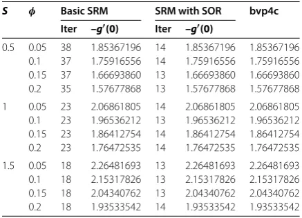
Table 6 Comparison of –g(0) obtained by bvp4c and SRM for different values of nanoparticle volume fraction with CuO-water nanofluid for fixed values ofPr= 6.7850,D= 1,r1= 2, m= 1.5,ω= 0.75 andNR= 1
S φ Basic SRM SRM with SOR bvp4c
Iter –g(0) Iter –g(0)
0.5 0.05 38 1.85367196 14 1.85367196 1.85367196 0.1 37 1.75916556 14 1.75916556 1.75916556 0.15 37 1.66693860 13 1.66693860 1.66693860 0.2 35 1.57677868 13 1.57677868 1.57677868 1 0.05 23 2.06861805 14 2.06861805 2.06861805 0.1 23 1.96536212 13 1.96536212 1.96536212 0.15 23 1.86412754 14 1.86412754 1.86412754 0.2 23 1.76472535 14 1.76472535 1.76472535 1.5 0.05 18 2.26481693 13 2.26481693 2.26481693 0.1 18 2.15317826 13 2.15317826 2.15317826 0.15 18 2.04340762 13 2.04340762 2.04340762 0.2 18 1.93533542 14 1.93533542 1.93533542
can be accelerated by the thermal dispersion. The thermal dispersion may be regarded as the effect of mixing to enhance heat transfer in the medium. Table further gives a comparison of the SRM and the bvpc results in the caseφ= . The spectral relaxation method converges to the numerical solutions for all parameter values matching the bvpc results up to nine significant digits.
Tables and show the skin friction coefficient and heat transfer rate for various physi-cal parameters in the case of a CuO-water nanofluid. The skin friction coefficient and the local Nusselt number are more influenced by the nanoparticle volume fraction than the type of nanoparticles. This observation is in agreement with Oztop and Abu-Nada []. In addition, water has the lowest skin friction coefficient and the local Nusselt number compared with CuO, AlO, TiO nanofluids. We observe that the skin friction
Table 7 Comparison of –f(0) obtained by bvp4c and SRM for different values of nanoparticle volume fraction with Al2O3-water nanofluid for fixed values ofPr= 6.7850,r1= 2,m= 1.5 and
ω= 0.75
Quantity φ Basic SRM SRM with SOR bvp4c
Iter –f(0) Iter –f(0)
NR= 1
S= 1
D= 1
0.05 23 1.32762309 14 1.32762309 1.32762309 0.1 23 1.31890045 14 1.31890045 1.31890045 0.15 23 1.29654739 13 1.29654739 1.29654739 0.2 23 1.26231187 14 1.26231187 1.26231187
NR= 5
S= 1
D= 2
0.05 23 1.32762309 14 1.32762309 1.32762309 0.1 23 1.31890045 14 1.31890045 1.31890045 0.15 23 1.29654739 14 1.29654739 1.29654739 0.2 23 1.26231187 13 1.26231187 1.26231187
NR= 10
S= 0.5
D= 5
0.05 38 1.17348812 14 1.17348812 1.17348812 0.1 38 1.16577817 14 1.16577817 1.16577817 0.15 37 1.14602026 14 1.14602026 1.14602026 0.2 37 1.11575944 13 1.11575944 1.11575944
Table 8 Comparison of –g(0) obtained by bvp4c and SRM for different values of nanoparticle volume fraction with Al2O3-water nanofluid for fixed values ofPr= 6.7850,r1= 2,m= 1.5 and
ω= 0.75
Quantity φ Basic SRM SRM with SOR bvp4c
Iter –g(0) Iter –g(0)
NR= 1
S= 1
D= 1
0.05 23 2.07754148 14 2.07754148 2.07754148 0.1 23 1.98429513 14 1.98429513 1.98429513 0.15 23 1.89386696 13 1.89386696 1.89386696 0.2 23 1.80581775 14 1.80581775 1.80581775
NR= 5
S= 1
D= 1
0.05 23 2.43674192 14 2.43674192 2.43674192 0.1 23 2.35621359 14 2.35621359 2.35621359 0.15 23 2.27587972 14 2.27587972 2.27587972 0.2 23 2.19532143 13 2.19532143 2.19532143
NR= 10
S= 1
D= 1
0.05 23 2.49509121 13 2.49509121 2.49509121 0.1 23 2.41787850 14 2.41787850 2.41787850 0.15 23 2.34049758 13 2.34049758 2.34049758 0.2 23 2.26250267 14 2.26250267 2.26250267
Tables and show the skin friction and heat transfer coefficients for various values of nanoparticle volume fraction and physical parameters. We note that the physical parame-tersNRandDhave no direct effect on the skin friction coefficient, but that the skin friction decreases with an increase in the unsteadiness parameter. From Table we observe that an increase in the thermal radiation parameter produces significant increases in the heat transfer coefficient. The skin friction and heat transfer rates decrease with an increase in the nanoparticle volume fraction.
The effects of the unsteadiness parameter, various nanoparticles, thermal dispersion and radiation parameters on various fluid dynamic quantities are shown in Figures -.
Figure 1 (a) Velocity and (b) temperature profiles forPr= 6.7850,NR= 1,D= 1,r1= 2,m= 1.5.
Figure 2 (a) Velocity and (b) temperature profiles forPr= 6.7850,NR= 1,D= 1,r1= 2,m= 1.5,S= 0.5,
φ= 0.2.
Figure shows the velocity and temperature distributions for different nanofluids. It can be observed that the velocity and temperature distributions for different nanoparti-cles increase gradually far from the surface of the stretching sheet. The fluid velocity and temperatures in the case of a CuO-water nanofluid are less than those in TiO-water and
AlO-water nanofluids.
Figure 3 Temperature profiles for (a)Pr= 6.7850,S= 0.5,NR= 1,r1= 2,m= 1.5 and (b)Pr= 6.7850,
S= 0.5,D= 1,r1= 2,m= 1.5.
Figure 4 (a) Skin friction and (b) heat transfer coefficients as a function of nanoparticle volume fraction, whenPr= 6.7850,S= 0.5,D= 1,NR= 1,r1= 2,m= 1.5.
Figure shows the skin friction coefficient as a function of the nanoparticle volume frac-tion. The skin friction coefficient increases with increasing nanoparticle volume fracfrac-tion. The maximum value of the skin friction in the case of a TiO-water nanofluid is attained
at higher values ofφin comparison with CuO-water and AlOnanofluids. Further, we
observe that a CuO-water nanofluid gives a higher drag force in opposition to the flow as compared to the other nanofluids. From Figure (b) we observe that the wall heat transfer rates for the nanofluids are increasing functions ofφ. A TiO-water nanofluid has higher
wall heat transfer rate as compared to the other nanofluids.
Figure 5 (a) Skin friction and (b) heat transfer coefficients as a function ofNR, whenPr= 6.7850,D= 1, r1= 2,m= 1.5.
Figure 6 (a) Skin friction and (b) heat transfer coefficients as a function ofD, whenPr= 6.7850,NR= 1, r1= 2,m= 1.5.
7 Conclusions
Competing interests
The authors declare that they have no competing interests.
Authors’ contributions
The work including proof reading was done by all the authors.
Acknowledgements
The authors are grateful to the reviewers for their comments and constructive suggestions. We acknowledge financial support from the University of KwaZulu-Natal.
Received: 18 June 2013 Accepted: 24 September 2013 Published:18 Nov 2013
References
1. Crane, LJ: Flow past a stretching plate. Z. Angew. Math. Phys.21, 645-647 (1970)
2. Gupta, PS, Gupta, AS: Heat and mass transfer on a stretching sheet with suction or blowing. Can. J. Chem. Eng.55, 744-746 (1977)
3. Sakiadis, BC: Boundary-layer behavior on continuous solid surfaces: I. Boundary-layer equations for two-dimensional and axisymmetric flow. AIChE J.7, 26-28 (1961)
4. Cortell, R: Effects of viscous dissipation and work done by deformation on the MHD flow and heat transfer of a viscoelastic fluid over a stretching sheet. Phys. Lett. A357, 298-305 (2006)
5. Hayat, T, Sajid, M: Analytic solution for axisymmetric flow and heat transfer of a second grade fluid past a stretching sheet. Int. J. Heat Mass Transf.50, 75-84 (2007)
6. Liao, SJ: On the analytic solution of magnetohydrodynamic flows of non-Newtonian fluids over a stretching sheet. J. Fluid Mech.488, 189-212 (2003)
7. Xu, H: An explicit analytic solution for convective heat transfer in an electrically conducting fluid at a stretching surface with uniform free stream. Int. J. Eng. Sci.43, 859-874 (2005)
8. El-Aziz, MA: Thermal-diffusion and diffusion-thermo effects on combined heat and mass transfer by hydromagnetic three-dimensional free convection over a permeable stretching surface with radiation. Phys. Lett. A372, 263-272 (2007)
9. El-Aziz, MA: Thermal radiation effects on magnetohydrodynamic mixed convection flow of a micropolar fluid past a continuously moving semi-infinite plate for high temperature differences. Acta Mech.187, 113-127 (2006) 10. Raptis, A: Flow of a micropolar fluid past a continuously moving plate by the presence of radiation. Int. J. Heat Mass
Transf.41, 2865-2866 (1998)
11. Mahmoud, MAA: Thermal radiation effects on MHD flow of a micropolar fluid over a stretching surface with variable thermal conductivity. Physica A375, 401-410 (2007)
12. El-Aziz, MA: Radiation effect on the flow and heat transfer over an unsteady stretching sheet. Int. Commun. Heat Mass Transf.36, 521-524 (2009)
13. Telles, RS, Trevisan, OV: Dispersion in heat and mass transfer natural convection along vertical boundaries in porous media. Int. J. Heat Mass Transf.36, 1357-1365 (1993)
14. Choi, SUS: Enhancing thermal conductivity of fluids with nanoparticles. In: Proceedings of the ASME International Mechanical Engineering Congress and Exposition, pp. 99-105. ASME FED231/MD66, San Francisco, USA (1995) 15. Masuda, H, Ebata, A, Teramae, K, Hishinuma, N: Alteration of thermal conductivity and viscosity of liquid by dispersing
ultra-fine particles. Dispersion of Al2O3, SiO2and TiO2Ultra-Fine Particles. Netsu Bussei4, 227-233 (1993)
16. Das, S, Putra, N, Thiesen, P, Roetzel, W: Temperature dependence of thermal conductivity enhancement for nanofluids. J. Heat Transf.125, 567-574 (2003)
17. Xuan, Y, Li, Q: Investigation on convective heat transfer and flow features of nanofluids. J. Heat Transf.125, 151-155 (2003)
18. Trisaksri, V, Wongwises, S: Critical review of heat transfer characteristics of nanofluids. Renew. Sustain. Energy Rev.11, 512-523 (2007)
19. Wang, XQ, Mujumdar, AS: Heat transfer characteristics of nanofluids: a review. Int. J. Therm. Sci.46, 1-19 (2007) 20. Kang, HU, Kim, SH, Oh, JM: Estimation of thermal conductivity of nanofluid using experimental effective particle
volume. Exp. Heat Transf.19, 181-191 (2006)
21. Velagapudi, V, Konijeti, RK, Aduru, CSK: Empirical correlations to predict thermophysical and heat transfer characteristics of nanofluids. Therm. Sci.12, 27-37 (2008)
22. Rudyak, VY, Belkin, AA, Tomilina, EA: On the thermal conductivity of nanofluids. Tech. Phys. Lett.36, 660-662 (2010) 23. Hady, FM, Ibrahim, FS, Abdel-Gaied, SM, Eid, MR: Radiation effect on viscous flow of a nanofluid and heat transfer
over a nonlinearly stretching sheet. Nanoscale Res. Lett.7, 229 (2012)
24. Olanrewaju, PO, Olanrewaju, MA, Adesanya, AO: Boundary layer flow of nanofluids over a moving surface in a flowing fluid in the presence of radiation. Int. J. Appl. Sci. Tech.2, 274-285 (2012)
25. Mahdy, A: Unsteady mixed convection boundary layer flow and heat transfer of nanofluids due to stretching sheet. Nucl. Eng. Des.249, 248-255 (2012)
26. Narayana, M, Sibanda, P: Laminar flow of a nanoliquid film over an unsteady stretching sheet. Int. J. Heat Mass Transf. 55, 7552-7560 (2012)
27. Kameswaran, PK, Narayana, M, Sibanda, P, Murthy, PVSN: Hydromagnetic nanofluid flow due to a stretching or shrinking sheet with viscous dissipation and chemical reaction effects. Int. J. Heat Mass Transf.55, 7587-7595 (2012) 28. Motsa, SS, Makukula, ZG: On spectral relaxation method approach for steady von Karman flow of a Reiner-Rivlin fluid
with Joule heating, viscous dissipation and suction/injection. Cent. Eur. J. Phys.11, 363-374 (2013)
29. Motsa, SS: A new spectral relaxation method for similarity variable nonlinear boundary layer flow systems. Chem. Eng. Commun. (2013). doi:10.1080/00986445.2013.766882
30. Tiwari, RK, Das, MK: Heat transfer augmentation in a two sided lid driven differentially heated square cavity utilizing nanofluids. Int. J. Heat Mass Transf.50, 2002-2018 (2007)
32. Guerin, CA, Mallet, P, Sentenac, A: Effective-medium theory for finite-size aggregates. J. Opt. Soc. Am. A23, 349-358 (2006)
33. Oztop, HF, Abu-Nada, E: Numerical study of natural convection in partially heated rectangular enclosures filled with nanofluids. Int. J. Heat Fluid Flow29, 1326-1336 (2008)
34. Canuto, C, Hussaini, MV, Quarteroni, A, Zang, TA: Spectral Methods in Fluid Dynamics. Springer, Berlin (1988) 35. Trefethen, LN: Spectral Methods in MATLAB. SIAM, Philadelphia (2000)
36. Singh, P, Jangid, A, Tomer, NS, Sinha, D: Effects of thermal radiation and magnetic field on unsteady stretching permeable sheet in presence of free stream velocity. Int. J. Inf. Math. Sci.6, 160-166 (2010)
10.1186/1687-2770-2013-242
![Table 1 Thermophysical properties of water and nanoparticles, Oztop and Abu-Nada [33]](https://thumb-us.123doks.com/thumbv2/123dok_us/501722.2049325/6.595.205.388.98.155/table-thermophysical-properties-water-nanoparticles-oztop-abu-nada.webp)