UNIVERSITY OF TRENTO
Department of Mathematics
PhD in Mathematics
XXVIII CYCLE
From data to mathematical analysis and
simulation in models in epidemiology and ecology
Advisor:
PhD student:
Prof. Andrea Pugliese
Valentina Clamer
Commitee members for defense of Ph.D dissertation: Prof. Gianpaolo Scalia Tomba (Second University of Rome, Italy)
Prof. Marino Gatto (Politecnico Milano, Italy) Prof. Stefano Bonaccorsi (University of Trento, Italy)
Defense of Ph.D dissertation:
If I know what love is, it is because of you. — Herman Hesse
Contents
Introduction xvii
I
Estimating transmission probability in schools for
the 2009 H1N1 influenza pandemic in Italy
1
1 Introduction 3
2 Background on mathematical models 5
2.1 Deterministic models . . . 6
2.2 Stochastic models . . . 7
2.2.1 Background on stochastic systems . . . 7
2.2.2 A chain binomial model . . . 8
2.2.3 Methods . . . 8
2.3 Introduction to Monte Carlo Markov Chain . . . 9
2.3.1 The Metropolis-Hastings algorithm . . . 9
3 Methods 11 3.1 Data . . . 11
3.2 Epidemic model . . . 13
4 Parameters estimation 15 4.1 Basic reproduction number . . . 15
4.2 Tests on simulated data . . . 16
4.2.1 Test with missing data . . . 20
4.2.2 Test with missing data and errors . . . 21
4.3 Model variants . . . 21
4.4 Estimates of transmission probabilities . . . 23
4.5 Model validation . . . 24
vi CONTENTS
5 Discussion 27
A The algorithm used 33
A.1 Parameters updating . . . 34
II
Dynamics of Host-Parasitoid Interactions and
Co-existence of Different Hosts
37
1 Introduction 39 2 Background on population models 41 2.1 Classical models . . . 412.2 Delay differential equations . . . 42
2.2.1 Age structure models . . . 42
3 Model 45 4 Invasibility conditions 49 4.1 Single host equilibria . . . 49
4.2 Invasibility under periodic conditions . . . 54
4.3 Approximation of dominant eigenvalue . . . 60
4.4 Application to host-parasitoid model . . . 63
5 Discussion 65 A The characteristic equation 69 A.1 Density-dependence two hosts present . . . 72
III
Simulations of biological control through parasitoids
of Drosophila suzukii
73
1 Introduction 75 1.1 Biological background . . . 751.2 Experiments . . . 77
2 Methods 79 2.1 Two hosts-two parasitoids model . . . 79
CONTENTS vii 2.2 One host-one parasitoid model . . . 82 2.2.1 Equilibrium with no parasitoids . . . 83 2.3 Parameters extrapolation . . . 83
3 Preliminary results 87
3.1 Simulations . . . 87 3.1.1 Laboratory conditions . . . 87 3.1.2 Increased death rates . . . 93
4 Discussion 95
List of Figures
3.1 Daily number of new cases in school A (panel a) and in school B (panel b), as derived from the collected data. . . 12 4.1 Linear regression on cumulative infection data in school A (panel
a) and in school B (panel b). Black points were used in the linear regression procedure for estimating the epidemic growth rate. . . . 16 4.2 Estimates ofγ (panels a and c) and ofqc(panels b and d) in 9 sets of
simulations performed by varyingγandqcwhile keepingR0 ≈1.48
(in Table 4.1). Panels a) and b) have n= 25, c) and d) have n= 250. The reference values used in the simulations are represented as white dots, while the means of the posterior distribution are represented as black dots, with the bars representing 95%-credible intervals. . . 18 4.3 (a) Ten sets of 50 simulations starting from reference values
repre-sented as white dots (in Table 4.2) and ε= 10−3. The estimated values are represented as black dots with the 95%-credible intervals (b) Fraction of simulations for which the 95%-credible intervals for
the different parameters do not intersect. . . 20 4.4 Fifty simulations (panels a and c) starting from reference values
represented by white dots (in Table 4.2) and ε= 10−3 by assuming that a 20% of the data of each class is not reported. The estimated values are represented as black dots with the 95%-credible intervals. Fraction of simulations in which the 95%-credible intervals for the different parameters do not intersect in panels b) and d). In panels a) and b) 20% of the data are considered to be missing. In panels c) and d) 20% of the data of each class are not regarded and only the 70% of the data are correct, the 20% of them correspond to a
±1 and the remaining 10% to a ±2. . . 22
LIST OF FIGURES ix 4.5 Estimated values of the transmission parameters for school A and
B. White and black dots represent the mean of the posterior dis-tribution for school A and school B respectively, bars represent 95%-credible intervals. (b) Estimated values of the basic repro-duction number R0 inside schools A and B. Thick line and bars represent means and 95%-credible intervals. . . 24 4.6 The plot of the total number of infectious individuals (panel a)
and the duration of the epidemic (panel b) in 400 simulations. The black dot indicates the observed number of infectious individuals and the observed length of the epidemic in the two schools. Thick line and bars represent means and 95%-credible intervals. . . 25 4.1 Eigenvalues at Hopf bifurcation for dA1 = dHB1 ≈ 0.3089 and
ρ1 = 5 (left) and periodic solutions for dA1 = 0.35 and ρ1 = 5
(right) of Host 1 for the parameters values in Table 4.2. . . 56 4.2 The thick line represents the boundary that divides the (dA2, ρ2
)-plane into stable and unstable regions by having fixed ρ1 = 5,
dA1 = 0.35. The straight dashed line represent instead the value
ρ1e−
νLdP TL
αsP that comes from (4.7). . . . 57 4.3 For ρ1 = 5, and dA1 = dA2 = var, when dA > dHB, host 2 can
invade for ρ2 >ρ¯(dA), a decreasing function of dA, and host 1 can
invade for ρ1 <ρˆ(dA), an increasing function ofdA. . . 58
4.4 The thick curve represents the condition for invasibility of the host 2 periodic solution with ρ1 = 5,dA1 = 0.3 and νL1 = νL2 = 0.
The solid thick curve represents instead the boundary that divides the (dA2, ρ2)-plane into stable and unstable regions, below which
coexistence is not possible. The dotted thin curve is the bifurcation curve of the equilibrium Eq2: the right curve part is the locus of the Hopf bifurcations leading to periodic solutions; the bottom segment is the locus of trans critical bifurcation with the trivial equilibrium. . . 60 3.1 Under laboratory conditions simulations. Panel (a), (b), (c) and
(d) represent the case with an initial adult parasitoid value equal to 10% of adult hosts, in 500 days with attack rates 10α,α4,α2, α
respectively. . . 89 3.2 Under laboratory conditions simulations when no parasitoids are
x LIST OF FIGURES
3.3 Under laboratory conditions simulations with an initial adult parasitoid value equal to 10% of adult hosts introduced at time
x= 20, in 500 days with attack rates 10α. . . 91 3.4 Under laboratory conditions simulations. Panel (a), (b), (c) and
(d) represent the case with an initial adult parasitoid constant value equal to 0.5, in 500 days introduced when host population is at equilibrium with attack rates 10α,α4,α2, α respectively. . . 92 3.5 Increased death rates. Panel (a) and (b) represent the case with
List of Tables
3.1 Collected data. Summary of the main features emerging from the questionnaires collected in schools A and B in Trento, Italy in 2009. 12 3.2 Model parameters and variables. Description of the notation used. 14 4.1 Parameter values for the probability of remaining infective for two
days γ, and the class infection probability qc used in the 9 sets of
simulations as to have R0 ≈1.48 with a class of n= 25 students
and the fictional case of a class of n= 250 students. . . 17 4.2 Parameter values of the class infection probability qc, the grade
infection probabilityqg and the school infection probabilityqs used
in the 10 sets of simulations. . . 19 4.3 DIC values of the different models considered. Model CGS has
three different transmission rates inside the school (qc, qg andqs) .
Model S has a homogeneous infection rate inside the school (qc).
Model CS has a transmission rate for the class (qc) and a different
transmission rate in the remaining part of the school (qg). Model
CGSvar is the same as CGS but with with a non-constant ε. . . . 23 4.4 Mean and 95%-credible intervals of the estimates for the infection
probabilities in schools A and B, when considering model CGS. . 23 3.1 Model parameters present in the 2 host-parasitoid model. All
parameters are kept constant and density-independent except the larval death rate dLi(Li(t)) = µLi +νLiLi(t) that depends on a constant background mortality, µLi, and on the quantity for which the pro capita mortality changes by adding a new individual, νLi. 47 4.1 Parameter values used in the computation. We analyse the case
when two hosts are identical except for the adult host mortality
dA and the fecundity ρ. . . 55
xii LIST OF TABLES
4.2 Parameter values used to compute a distinct periodic solution for
dA1 = 0.35. . . 57
2.1 Model parameters present in the two hosts-two parasitoids model. All parameters are kept constant and density-independent except of the larval death rate that depends on larvae density. . . 81 2.2 Model parameters present in the one host-one parasitoid model.
All parameters are kept constant and density-independent except of the larval death rate that depends on larvae density. . . 84 2.3 Parameter extrapolated from [110, 144] used to see parasitoids
impact on a host population at equilibrium. . . 86 3.1 Time needed by parasitoids to halve host pupae under different
combinations of attack rate and percentage of introduced parasitoids. 88 3.2 Parameters obtained by considering that probably in nature death
rates both of hosts and of parasitoids can be higher than the rates obtained under laboratory conditions. . . 93 3.3 Time needed by parasitoids to obtain 50 host pupae under
Abstract
This dissertation is divided into three different parts.
In the first part we analyse collected data on the occurrence of influenza-like illness (ILI) symptoms regarding the 2009 influenza A/H1N1 virus pandemic in two primary schools of Trento, Italy. These data were used to calibrate a discrete-time SIR model, which was designed to estimate the probabilities of influenza transmission within the classes, grades and schools using Markov Chain Monte Carlo (MCMC) methods. We found that the virus was mainly transmitted within class, with lower levels of transmission between students in the same grade and even lower, though not significantly so, among different grades within the schools. We estimated median values of R0 from the epidemic curves in the two
schools of 1.16 and 1.40; on the other hand, we estimated the average number of students infected by the first school case to be 0.85 and 1.09 in the two schools. This discrepancy suggests that household and community transmission played an important role in sustaining the school epidemics. The high probability of infection between students in the same class confirms that targeting within-class transmission is key to controlling the spread of influenza in school settings and, as a consequence, in the general population.
In the second part, by starting from a basic host-parasitoid model, we study the dynamics of a 2 hosts-1 parasitoid model assuming, for the sake of sim-plicity, that larval stages have a fixed duration. If each host is subjected to density-dependent mortality in its larval stage, we obtain explicit conditions for coexistence of both hosts, as long as each 1 host-parasitoid system would tend to an equilibrium point. Otherwise, if mortality is density-independent, under the same conditions host coexistence is impossible. On the other hand, if at least one of the 1 host-parasitoid systems has an oscillatory dynamics (which happens under some parameter values), we found, through numerical bifurcation, that coexistence is favoured. It is also possible that coexistence between the two hosts
xiv LIST OF TABLES
occurs even in the case without density-dependence. Analysis of this case has been based on methods of approximation of the dominant characteristic multi-pliers of the monodromy operator using a recent method introduced by Breda et al. Models of this type may be relevant for modelling control strategies for Drosophila suzukii, a recently introduced fruit fly that caused severe production losses, based on native parasitoids of indigenous fruit flies.
The essence of mathematics is not to make simple things complicated, but to make complicated things simple.
— S. Gudder
Acknowledgements
I would like to thank my advisor, Prof. Andrea Pugliese, for his teaching and support and all the people with whom I had useful discussions about this work.
I thank the headmasters of the primary schools of Povo and Villazzano, Trento (Italy) for permitting us to run the survey and the students’ parents and carers for their participation. I am grateful to Prof. Mimmo Iannelli and Antonella Lunelli for their collaboration in the design and distribution of the questionnaire and digitalization of the data, to Caterina Rizzo for her help in designing the questionnaire and for providing the InfluNet data.
I thank Valerio Rossi Stacconi for providing the data on Drosophila suzukii and its parasitoids and Prof. Dimitri Breda and Davide Liessi for their collabora-tion in finding numerically coexistence condicollabora-tions with periodic solucollabora-tions. I am grateful to the Lexem Project that financially supported part of this thesis.
Last but not least, I would also like to thank my family, the loves of my life and all my friends for their support, patience and smiles during the last three years of my life, even when I was mostly stressed. You make me happy.
V. C.
Introduction
T
his Ph.D dissertation summarizes the results of two different works. The research of the first topic during my Ph.D program originates from a result first presented in my Master thesis and presented here in a developed version, the analysis of collected data on the 2009 influenza A/H1N1 virus pandemic in two primary schools of Trento, Italy, using Markov Chain Monte Carlo (MCMC) methods.The choice of the second topic is due to an offer that was made to me less than two years ago that has intrigued me. This offer consisted in a collaboration with the Edmund Mach Foundation to the Lexem Project that aims at producing new strategic knowledge and innovative tools useful for supporting decision-making for what concerns the crop pest Drosophila suzukii. In fact, since its first detection in 2008, D. suzukii has provoked serious damages to orchards causing significant economic losses and this has revived the interest in understanding multi-hosts multi-parasitoids interactions.
Even if the two parts that constitute this thesis are very different one from the other, we can find a leitmotiv that links their topics, mathematical modelling. Mathematical models are in fact a useful tool to simulate epidemic spread scenarios or dynamics that result from the interactions of different species, and can be a significant help for public health policies decisions. Formulation of a model depends indeed on the aspects chosen by the modeller, and, for this reason, it can easily be used to analyse different real-life situations and can be applied to different fields of study such as biology, epidemiology, demography, finance . . .
Part I focusses on the study of a discrete-time SIR model.
This part has been inspired by a real outbreak that occurred in two primary schools in the province of Trento, Italy, in 2009. Parameters estimation
xviii INTRODUCTION
in such a situation is a key part of the modelling process and Bayesian inference has been performed in this thesis.
The modelling framework presented here constitutes a novel approach that can be applied to different infections detected in many countries.
In this Part we present a brief overview of mathematical models used in epidemiology and on Markov Chain Monte Carlo methods. Then we analyse data collected in two primary schools in the province of Trento, Italy, with an epidemic discrete-time SIR model, where the transmission parameters are estimated via Markov chain Monte Carlo methods. Last, we apply different parameters estimations. We start with a basic concept that characterize epidemiology, the basic reproduction number, and then we apply a developed model that is based on three different kinds of interactions: within class, grade and school. The first test on simulated data that we have performed refers to a simple case of a single class with different class sizes, aiming at the estimate of the probabilities to remain infectious for two days and to be infected from someone inside the class. Then we test the model and the estimation algorithm under different parametrizations. We compare three variants of the model using an adapted version of the deviance information criterion. Finally, we validate the presented model and estimate model parameters in the two selected primary schools. Part II of this dissertation looks at the dynamics that result from the
interac-tions of different species.
xix
on biological motivations for our study and on classical population models that provide the model prototype of host-parasitoid models. Then we introduce a 2 host-parasitoid model based on delay differential equation that is an extension of a model already presented in the literature. In this model we consider that adult parasitoids can attack only host larvae (adult hosts are invulnerable to parasitism) whose mortality can depend or not on their density at time t. We give coexistence condition of the presented model that are found by linearising the system around the equilibria with only one host species present. We show that, when no density-dependence is present, the two hosts cannot coexist but, once density-dependence is introduced, we can find some conditions for hosts coexistence. Last, we discuss also what happens if we are in periodic conditions using numerical approximations and we give a mathematical proof of what we have found through the analysis.
Part III summarizes the first results of a topic that we started working on recently, application of the model to raw data.
In particular, we present the experiments conducted by Tochen et al. and Stacconi et al. that can be considered useful to apply the presented model to raw data. However, we have to keep in mind that field and semi field experiments were performed late in the season and thus the obtained value are not reliable and are not use in these preliminary simulations.
Part I
Estimating transmission
probability in schools for the
2009 H1N1 influenza pandemic
in Italy
Chapter 1
Introduction
I
n this chapter we give an introduction to epidemic models. These mod-els are in fact being extensively used to understand the main pathways of spread of infectious diseases, and thus to assess control methods. In particular, we present a brief overview of what has been done and used in this work.Generally, epidemic models are fitted to rather aggregated datasets reporting number of new cases (possibly stratified by age or other variables of interest) in each time interval (often a week, although sometimes daily reports are available, especially at the initial outbreak of an infection). In some cases, data on all individuals of a small community have been available [1], and this has allowed to obtain a better understanding of the person-to-person spread. Still, the question rises of whether small isolated communities are representative of disease spread in more usual contexts.
The attention that was given to the A/H1N1 2009 flu pandemic has made it possible to collect detailed data on the epidemic spread in more typical contexts. Schools are well known to represent hot spots for epidemic spread, as can be seen in [2–13]. Contact rates within schools are generally higher than outside, as was also noticed in [3, 14, 15]. Using detailed data on an outbreak of 2009 pandemic influenza in a school, Cauchemez et al. [16] estimated the different infection probabilities within each class, or grade, and in the whole school, as well as quantified the spread through other household members, and were also able to assess the role of heterogeneities in contact rates.
In this work we provide estimates for transmission rates of 2009 A/H1N1 pandemic influenza at the three levels of class, grade and school by analysing
4 CHAPTER 1. INTRODUCTION
data on the occurrence of influenza-like illness (ILI) symptoms among pupils of two primary schools in Trento (Italy). The data were collected retrospectively in December 2009, a few weeks after the epidemic peak, through a questionnaire delivered to the parents of the pupils attending the two primary schools. As far as we know, this is the first case in Italy, and one of the first in Europe, in which influenza transmission is estimated in a school. The estimates appear consistent between the two schools and with the general understanding of influenza transmission.
We developed a discrete-time SIR model to analyse the collected data, where the transmission parameters were then estimated via Markov chain Monte Carlo methods, appropriate to make parameter inference in presence of missing data [17, 18].
In order to understand the power of the method, we applied the algorithm also to synthetic data, generated to reproduce a school structure, under several hypotheses on the transmission dynamics. This work on synthetic data made us, on the one hand, get a better interpretation of the results obtained, showing for instance to which degree parameters are identifiable; on the other hand, assess the loss in accuracy resulting from missing data and other sources of error.
Chapter 2
Background on mathematical
models
T
his chapter summarizes some preliminaries on mathematical models gen-erally used in epidemiology and on Markov Chain Monte Carlo methods that would be useful for the analysis of the transmission probabilities in schools for the 2009 H1N1 influenza pandemic in Italy. This is in fact one of the main characteristic of epidemiology that wants to understand the complex mechanisms behind an observed outbreak to try to control it using mathematical models [19–21].When we consider epidemics within a population, traditionally we focus on the dynamics among individuals of the population and not on the process that occurs within a single component of the community at a pathogen level. In fact, since we are interested in the number of infected individuals and in the infection spread, we can disregard the mechanisms inside an individual that make him sick. Hence, when we describe an epidemic at the population level, we can distinguish three main categories in which to divide the population: susceptibles (healthy and infectable individuals), infectives (infected and infectious individuals) and removed (usually immune individuals after recovery). The first mathematical models appeared at the beginning of the 20th century [22–28]. In particular, Kermack and McKendrick in [26–28] laid the foundations of one of the most relevant mathematical frameworks for epidemic description in this field, the SIR model. In their paper that differs in the interpretation from the one present in this dissertation, Kermack and McKendrick includes into the removed not only immune individual but also dead or quarantined individuals because of the
6 CHAPTER 2. BACKGROUND ON MATHEMATICAL MODELS
infection.
By following the description of the epidemic given in these papers, the state of the population can be identified by three basic variables: S(t), the number of susceptibles at time t, I(t), the number of infectives at time t and R(t), the number of removed at time t. As we have said previously, these are only the foundations to describe an epidemic. In fact, actually, there may be other characterizing classes, for instance exposed (infected individual that are not infectious) or differently infectious infectives. However a general understanding of the problem can be obtained by considering only the three main class introduced above.
After the division of the population into epidemiological classes, both deter-ministic or stochastic models can be used. The choice between them follows from the size of the population taken into account. In fact, one of the main assumption in deterministic population models is that the population has to be very large, otherwise epidemic models fail to catch the random nature of transmission events. In the following Section we present and discuss briefly similarities and differences between these two different models. However, generally, when an epidemic is described, we have to distinguish if the disease taken into account impart lifelong immunity or not. In the first case we have the so called SIR models, in the latter SIS or SIRS (according to the presence of a transitory immunity or not).
2.1
Deterministic models
A deterministic model is characterized by the fact that, once initial conditions and parameter values are fixed, its evolution is uniquely determined. This kind of models has been used to understand a huge variety of situations such as parameters estimation and surveillance data fitting [29–31], control measures impact assessment [32], antibiotic use investigation [33] or transmission dynamics analysis [34–37].
Even if deterministic models are easy to simulate and analyse, when low levels of infections or small populations are present or when the whole epidemic outbreak is not observed, this kind of model fails to catch the random nature of transmission events.
2.2. STOCHASTIC MODELS 7
2.2
Stochastic models
Differently from deterministic models, stochastic models are based on prob-abilities on the occurrence of a certain event. Thus, the study of temporal evolution of such a model is more complex than the study of a deterministic model and, for this reason, computer simulations are very useful.
2.2.1
Background on stochastic systems
In this dissertation we analyse a pandemic that occurred in two primary schools of Trento, Italy. Analysing data from infectious diseases is a non-standard problem and the inference problems are complicated because these data are highly dependent, incomplete data that come from only partially observable real-life situations. However it is possible to develop a simple stochastic model that has to be a close approximation of the real system considered. The model that we take into account and that can be used as a starting point for inference tries to imitate the behaviour of this system by studying the interactions among the pupils of a primary school. These interactions can be divided into internal relationships that connect pupils within the school, and external relationships that connect pupils with the world outside the school.
The importance of a model to study a system has been discussed by Rosenbluth and Wiener [38], who wrote:
No substantial part of the universe is so simple that it can be grasped and controlled without abstraction. Abstraction consists in replacing the part of the universe under consideration by a model of similar but simpler structure. Models . . . are thus a central necessity of scientific procedure.
After model formulation it is usual to perform a lot of simulations that can be regarded as statistical experiments, to keep track of parameters of interest and, at the end, to ensure that there is enough confidence in the results. Naylor et al. [39] wrote that:
8 CHAPTER 2. BACKGROUND ON MATHEMATICAL MODELS
A model that can describe the epidemic process in a real-life situation is the chain binomial model.
2.2.2
A chain binomial model
By following the previous assumptions on population division into epidemio-logical classes, we assume that the probability that a susceptible escapes infection when exposed to the i infectives of a generation is qi, i= 1,2, . . .. For the sake
of simplicity, assume that there are no sub clinical infections (all infectives can be recognized) and that after the infection each individual acquires immunity. These assumptions led us to deduce that the number of individuals that remain susceptible isSt+1 =St−It+1, by knowing the initial values I0 =i0 andS0 = s0.
Thus, the probability of having x infectives at time t+ 1, by knowing that at time t there are s susceptibles and i infectives, is
P(It+1 =x|St=s, It=i) =
s!
x!(s−x)!p
x
iqis−x (2.1)
where pi = 1−qi.
Reed-Frost (related to [40]) and Greenwood [41] formulated two particular cases of the chain binomial model by making different assumptions on the way in whichqi depends on i.
In 1928 in a biostatistic lecture, Reed and Frost assumed that, when the disease transmission occurs through close person-to-person contacts,qi =q1i that means
that the probability of escaping infection when exposed to i infectives of one generation is equivalent to escaping infection when exposed to a single infective in each of i separate generations.
On the other side, in 1931 Greenwood assumed that, when the probability of infection depends more on the behaviour of one individual than on the environ-ment, qi =q, i= 1,2, . . . and q0 = 1. Thus the chance of infection is the same
when exposed to one infective as when more than one infective is present.
2.2.3
Methods
2.3. INTRODUCTION TO MONTE CARLO MARKOV CHAIN 9 all the informations about the parameters, is defined via Bayes’ Theorem as the normalized product of the prior density and the likelihood.
To summarize briefly this method, denote with D observed data and with ϑ
model parameters and missing data.
Formal inference requires a joint probability distribution P(D, ϑ) given by
P(D, ϑ) =P(D|ϑ)P(ϑ). (2.2) Thus, through Bayes theorem, by having observed D, the posterior distribution is
P(ϑ|D) = P(ϑ)P(D|ϑ)
P(D) =
P(ϑ)P(D|ϑ) R
P(ϑ)P(D|ϑ)dϑ. (2.3)
Since the integral at denominator can be regarded as a normalising constant to ensure that P(ϑ|D) is a proper density, (2.3) can be written as
P(ϑ|D)∝P(D|ϑ)P(ϑ). (2.4)
2.3
Introduction to Monte Carlo Markov Chain
One of the most important methodology to analyse real-life situations is the methodology of Monte Carlo Markov Chain (MCMC). Its name comes from the generation of a Markov chain using the previous sample value to randomly generate the next one. It was first described by Metropolis et al. [44] and later refined by other people including Hastings [45], Geman and Geman [46], Gelfand and Smith [47], Gelman and Rubin [48, 49], and Green [50].
MCMC methods try to solve the problem in obtaining samplers from some complex probability distribution that we can face with the integration. This would seem to provide the solution to our problem, but first we need to discover how to construct a Markov chain such that its stationary distribution π(.) is our distribution of interest. Constructing such a Markov chain is surprisingly easy.
2.3.1
The Metropolis-Hastings algorithm
The form due to Hastings in 1970 is a generalization of the method of Metropolis et al. using an arbitrary transition probability function q(Y|X) =
P(X →Y).
At each time t, the next state Xt+1 is chosen sampling Y from a proposal
distribution q(.|Xt) and the acceptance probability is given by
α(X, Y) = min
1, π(Y)q(X|Y) π(X)q(Y|X)
10 CHAPTER 2. BACKGROUND ON MATHEMATICAL MODELS
If Y is accepted, the next state will be Xt+1 =Y, if it is rejected Xt+1 =Xt.
To implement successfully this algorithm, we have to keep in mind that initial simulations, the so called burn-in period, have to be discarded since it would be unlikely that they come from the stationary distribution of interest. After that we have to decide if the chain is a well mixing chain by considering an acceptance probability A that will say us if the chain mixes well or not. This is defined as the number of iterations where new values are accepted out of a batch of iterations. By following [16, 51], the acceptance probability value for a good mixing is between 10% and 40%. However, it should be borne in mind that an optimal A does not necessary imply convergence to a stationary distribution, although poor A could be due to a lack of mixing and convergence. It is also possible to have high acceptance and very low convergence [52].
Chapter 3
Methods
T
his chapter presents the collected data of two primary schools in the province of Trento, Italy, and the epidemic discrete-time SIR model used to analyse these data, where the transmission parameters were then estimated via Markov chain Monte Carlo methods.3.1
Data
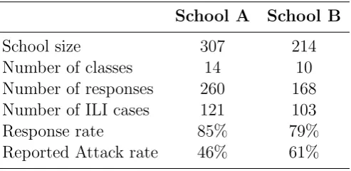
In December 2009 we delivered a questionnaire to the parents of the pupils of two primary schools in Povo (A) and Villazzano (B) in the province of Trento (Italy). School A consisted of 307 students divided into 14 classes of 5 different grades, while school B consisted of 214 students divided into 10 classes of 5 different grades. The questionnaire reported a description of ILI symptoms, asked the parents to report whether any member of the family had experienced ILI symptoms in the preceding months and, if that was the case, to report the date of symptoms onset (or an estimate of it) for each member of the family, similarly to what was done in [3, 4, 53]. Table 3.1 and Figure 3.1 summarize the data collected concerning the students of the two primary schools. The information provided on all the other members of the families were scarce and for this reason they were excluded from our study.
12 CHAPTER 3. METHODS
School A School B
School size 307 214
Number of classes 14 10 Number of responses 260 168 Number of ILI cases 121 103
Response rate 85% 79%
Reported Attack rate 46% 61%
Table 3.1: Collected data. Summary of the main features emerging from the
question-naires collected in schools A and B in Trento, Italy in 2009.
The overall response rate to the questionnaire was 82% (428/521) and the reported ILI cases were 224 (52%) (Table 3.1). In school A, the first two cases were reported on 16 October 2009 and the last case was reported 56 days later. In school B, the first case was reported on 10 October 2009 and the last case occurred 64 days later.
Figure 3.1 represents the number of new cases in the two schools and shows that most cases occurred within the central 30 days in school A, and even 20 days in school B.
date
ne
w cases in school A
0 2 4 6 8 12 (a)
16/10 5/11 25/11 11/12
10
14
date
ne
w cases in school B
0 2 4 6 8 12
16/10 5/11 25/11 11/12
10
14
(b)
Figure 3.1: Daily number of new cases in school A (panel a) and in school B (panel
3.2. EPIDEMIC MODEL 13
3.2
Epidemic model
The epidemic process is described using a discrete-time SIR model, with a time step of 1 day. Following [54], we assume that the incubation period (time from infection to symptom occurrence) is on average 2 days and varies between 1 and 3 days, and that the infectiousness profile is as described in [55]. This led us to do the following assumptions: if a child is infected at school on day t, he/she will be at school and infectious on dayt+ 1; on dayt+ 2 he/she will be infectious and either kept at home, or still at school with probability γ: from Figures 1b) and 1d) of [54] we estimateγ = 0.1. Hence, we assume that the school population can be divided into: susceptible individuals S, infectious individuals I (infected children who can transmit the disease, divided into two sub-compartments I1
and I2 depending on them being in the first or second day of infectiousness,
respectively) and recovered subjects R (including both recovered children and children kept at home after symptoms onset).
The model is a Markov chain where the individual transitions are given by
S →I1, I1
γ
→I2 I1 1−γ
→ R I2
1
→R.
The transition S→I1 depends on the infectious population. For the sake of
sim-plicity, we assume that I1 andI2 individuals are equally infectious. Furthermore,
by following [16], we assume different probabilities of infection: within-class (qc),
in the same grade but in a different class (qg), in the same school but in a different
grade (qs) and in households or in the general community (). We define
• Itj,h the number of infectious students (either in their first or second day of infectiousness) in grade j, class h at timet;
• It0j,h =P
k6=hI j,k
t the number of infectious students in the classes of grade j
other than h at time t
=Itj (number of infectious students in all classes of gradej)−Itj,h ;
• It00j =P
i6=j,hI i,h
t the number of infectious students in grades other than j
at time t
=It (number of infectious in all classes of the school) −Itj,
The probability for a susceptible student in gradej, classh to remain susceptible is
pj,ht = (1−qc)I
j,h t (1−q
g)I 0j,h t (1−q
s)I 00j
14 CHAPTER 3. METHODS
and 1−pj,ht is the probability of becoming I1 at timet+ 1.
Then the probability of having Stj,h+1 susceptibles at time t+ 1, by considering the school at timet, can be obtained as
P(Stj,h+1|Stj,h, Itj,h, Itj, It) =
Stj,h Stj,h+1
(pj,ht )Stj,h+1(1−pj,h
t )(S
j,h t −S
j,h
t+1) (3.2)
The full list of variables and parameters of the model is reported in Table 3.2. Model parameters have been estimated using MCMC methods, as described in [17, 56]. The estimated parameters are the infection probabilities within-class
qc, within the same grade qg, among different grades of the schools qs and from
outside the schools and the augmented data are all unobserved events such as the infection dates and the infection state of the children whose questionnaires were not filled (see Appendix A for further details).
Symbol Description
qc within-class infection probability
qg same grade infection probability
qs within-school infection probability
ε outside-school infection probability
γ probability to remain infective for two days
It number of infective subjects at time t in the whole school
Itj number of infective subjects at time t in grade j
Itj,h number of infective subjects at time t in grade j and class h Stj,h number of susceptible individuals at timet of gradej and class h nj number of classes of gradej
Chapter 4
Parameters estimation
W
e summarize in this part of the dissertation some different parameters estimations. We start with a basic concept that characterize epidemi-ology, the basic reproduction number and then we apply the model presented in Section 3.2, CGS (Class-Grade-School) model, to simulated data. The first test on simulated data in this chapter refers to a simple case of a single class with different class sizes, aiming at the estimate of the probabilities to remain infectious for two days and to be infected from someone inside the class. Then we test the model and the estimation algorithm under different parametrizations. We compare three variants of the model using an adapted version of the deviance information criterion and, finally, we estimate model parameters in schools A and B and we validate it.4.1
Basic reproduction number
A typical summary indicator of an epidemic is its basic reproduction number
R0, which represents the expected number of secondary cases generated by a
single typical infection in a completely naive population. The reproduction number estimated in this work is school-specific. R0 can be estimated through
the rate of initial epidemic growth r using the formula R0 = 1 +rTI [57], where
TI represents the mean generation time;r has been estimated through the fit of a
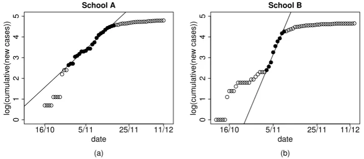
linear model either to the incidence data (grouped by 3 days) or to the cumulative number of cases (see [58] for a statistical analysis of the consequences of either choice) in the log-scale (Figure 4.1 shows the fit to the curve of cumulative cases over a specific time window).
16 CHAPTER 4. PARAMETERS ESTIMATION 0 1 2 3 4 5 School A date log(cum ulativ e(ne w cases)) (a)
16/10 5/11 25/11 11/12
0 1 2 3 4 5 School B date log(cum ulativ e(ne w cases)) (b)
16/10 5/11 25/11 11/12
Figure 4.1: Linear regression on cumulative infection data in school A (panel a) and
in school B (panel b). Black points were used in the linear regression procedure for estimating the epidemic growth rate.
We estimated the initial growth rate r both from the (grouped) incidence curve and from the cumulative curve (Figure 4.1), selecting those time windows in the growing part of the epidemic for whichR2 was sufficiently high (>0.95 for the cumulative curve,>0.7 for the incidence curve); assuming that the infectious period at schoolTI is 1.1 day, we obtained a median R0 of 1.16 for school A and
1.40 for school B; the overall range of confidence intervals (obtained from the different time windows) is 0.93-1.43 for school A; 1.08-1.76 for school B using the fit from incidence curves. The intervals obtained from cumulative curve are much narrower, but may be deceivingly so [58].
The classical definition ofR0 in a finite population stochastic model is generally
based on the limit as the population grows to infinity (see, for instance, [59]). Instead of doing this, we rely on a simple operational definition, namely we define
R0 as the average number of students infected by the first infected student in
the school. By assuming to havens grades (5 in Italian primary schools), each
with ng classes with n students, then we obtain
R0 = (qc(n−1) +qgn(ng−1) +qsnng(ns−1))(1 +γ). (4.1)
4.2
Tests on simulated data
4.2. TESTS ON SIMULATED DATA 17 We started with the simple case of a single class, aiming at the estimate of the probabilities to remain infectious for two days, γ, and to be infected from someone inside the same class, qc. We performed a series of simulations varyingγ
from 0.1 (the probability to remain infective for two days is very low) to γ = 0.9 (the probability to become an I2 is very high) with a step of 0.1; correspondingly,
qc is changed in such a way that R0 (in this case nqc(1 +γ)) remains constant.
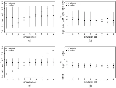
In Table 4.1 the parameters values from which we started are shown, both for a class of n= 25 children and for a (fictional) case of a class of 250 children. Figure 4.2 shows the results obtained in the case of a class of n= 25 children or in the (fictional) case of a class of 250 children.
Simulation n= 25 n = 250 set γ qc qc
1 0.1 0.054 0.0054 2 0.2 0.049 0.0049 3 0.3 0.046 0.0046 4 0.4 0.042 0.0042 5 0.5 0.039 0.0039 6 0.6 0.037 0.0037 7 0.7 0.035 0.0035 8 0.8 0.033 0.0033 9 0.9 0.031 0.0031
Table 4.1: Parameter values for the probability of remaining infective for two daysγ,
and the class infection probability qc used in the 9 sets of simulations as to
have R0 ≈1.48 with a class of n= 25 students and the fictional case of a
18 CHAPTER 4. PARAMETERS ESTIMATION
2 4 6 8
0.0 0.2 0.4 0.6 0.8 1.0 simulation set γ
1 3 5 7 9
(a)
γ reference
γ median
2 4 6 8
0.00 0.02 0.04 0.06 0.08 0.10 simulation set qc
1 3 5 7 9
qc reference
qc median
(b)
2 4 6 8
0.0 0.2 0.4 0.6 0.8 1.0 simulation set γ
1 3 5 7 9
(c)
γ reference
γ median
2 4 6 8
0.000
0.004
0.008
simulation set
qc
1 3 5 7 9
qc reference
qc median
(d)
Figure 4.2: Estimates of γ (panels a and c) and of qc (panels b and d) in 9 sets of
simulations performed by varying γ and qc while keeping R0 ≈1.48(in
Table 4.1). Panels a) and b) have n= 25, c) and d) have n= 250. The
reference values used in the simulations are represented as white dots, while the means of the posterior distribution are represented as black dots,
with the bars representing 95%-credible intervals.
It may be noticed that the mean value of estimated γ is always close to 0.5, independently of the value of γ used in simulations. Increasing n reduces the width of credible intervals, but does not remove the bias. Also the mean estimated value ofqc is almost constant, independently of the value used in the
simulations, at the value that would be correct for γ = 0.5.
4.2. TESTS ON SIMULATED DATA 19 We generated data under different parameter values, ranging from the case where
qc, qg and qs are approximately equal (transmission homogeneous among all
students in a school) to another one where qc = 10qs and qg is intermediate
(transmission is higher to students in the same class, then to those in the same grade, and lowest to all other students of the school). The parameter values have been chosen so as to have (using formula (4.1) of the main text)
R0 ≈1.48 [54, 60–62].
Precisely, we performed 10 sets (labelled 1 to 10) of 50 simulations with the parameter values shown in Table 4.2, and for each simulation we ran the MCMC algorithm to obtain a posteriori distribution of the parameters qc, qg, qs andε.
The results are shown in Figure 4.3 (panel a)).
It can be seen that the estimates are reasonably correct, with the mean of the posterior distributions around the reference values. It may be noticed, however, that, when the three parametersqc,qg andqsare close to each other, the algorithm tends to overestimate qc, the transmission rate in the same class.
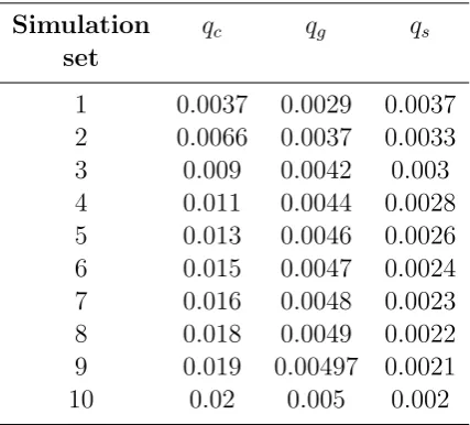
Simulation qc qg qs
set
1 0.0037 0.0029 0.0037 2 0.0066 0.0037 0.0033 3 0.009 0.0042 0.003 4 0.011 0.0044 0.0028 5 0.013 0.0046 0.0026 6 0.015 0.0047 0.0024 7 0.016 0.0048 0.0023 8 0.018 0.0049 0.0022 9 0.019 0.00497 0.0021 10 0.02 0.005 0.002
Table 4.2: Parameter values of the class infection probabilityqc, the grade infection
probability qg and the school infection probability qs used in the 10 sets of
20 CHAPTER 4. PARAMETERS ESTIMATION
An interesting question is whether the 95%-credible intervals for the three parameters intersect each other. The answers are shown in Figure 4.3 (panel b)). It can be seen that, when the parameters are indeed equal, around 5% of the times one obtains non-intersecting 95%-credible intervals, something close to expectations.
On the other hand, a difference is picked up almost always between qc and qs
from set 4 onwards (i. e. when the ratio qc/qs ≈ 3.8) and between qc and qg
from set 8 onwards (i. e. when the ratio qc/qg ≈ 3.7), while the ratio qg/qs
never reaches such values, and thus a difference between qg andqs is seen only
occasionally in the simulations. We found that the infection probabilitiesqc, qg,
2 4 6 8 10
0.00
0.02
0.04
simulation set
values
1 3 5 7 9
(a)
qc reference
qc median
qg reference
qg median
qs reference
qs median
2 4 6 8 10
0.0
0.4
0.8
simulation set
fr
action of disjointed CI
1 3 5 7 9
0.2
0.6
1.0
(b)
qc>qs
qc>qg
qg>qs
Figure 4.3: (a) Ten sets of 50 simulations starting from reference values represented
as white dots (in Table 4.2) and ε = 10−3. The estimated values are
represented as black dots with the 95%-credible intervals (b) Fraction of
simulations for which the 95%-credible intervals for the different
parame-ters do not inparame-tersect.
qs and ε were successfully identified .
4.2.1
Test with missing data
4.3. MODEL VARIANTS 21 wider than in the case without missing data, and thus they intersect somewhat more often. It can also be remarked that, with missing data, the transmission rate inside the class qc is on average overestimated in all simulation sets.
4.2.2
Test with missing data and errors
To see if the algorithm works also in the most general case in which some reported data are wrong, we consider that 20% of the data of each class are not regarded and that only the 70% of the data that we have are correct, the 20% of them correspond to a ±1 and the remaining 10% to a ±2 and we report the results in Figure 4.4 (panels c) and d)). Also in this case the estimation of the data is reasonably correct and this indicates that we have obtained a robust result, although the absolute value of qc is somewhat overestimated when the
parameters are close to each other.
4.3
Model variants
We considered the following two simplifications of the CGS model presented in Section 3.2: model CS (Class-School) where we differentiate between within-class transmission and within-school transmission only, without considering a separate probability of transmission within the same grades and model S (School only), where we assume that the probability of transmission is the same for all students in the school. We explore a further variant of model CGS (CGS-var), where the probability of infection from outside the school, instead of being constant over time, is assumed to be proportional (through a constant ε) to the ILI incidence at the corresponding week in the province of Trento, as reported by the surveillance system InfluNet of the Italian Institute of Health [63].
We compare the model variants using an adapted version of the deviance infor-mation criterion (DIC) described in [64, 65]. Specifically, distinguishing between actual model parameters (ϑ) and unobserved events (Y), we computed a marginal-ized DIC as
DIC =−4E(ϑ,Y)log (L(X, Y|ϑ)) + 2EY log L(X, Y|ϑ¯)
22 CHAPTER 4. PARAMETERS ESTIMATION
2 4 6 8 10
0.00 0.01 0.02 0.03 0.04 simulation set values (a) qc reference
qc median
qg reference
qg median
qs reference
qs median
2 4 6 8 10
0.0 0.2 0.4 0.6 0.8 1.0 simulation set fr
action of disjointed CI
(b) qc>qs
qc>qg
qg>qs
2 4 6 8 10
0.00 0.01 0.02 0.03 0.04 simulation set values (c) qc reference
qc median
qg reference
qg median
qs reference
qs median
2 4 6 8 10
0.0 0.2 0.4 0.6 0.8 1.0 simulation set fr
action of disjointed CI
1 3 5 7 9
0.2
0.6
1.0
(d) qc>qs
qc>qg
qg>qs
Figure 4.4: Fifty simulations (panels a and c) starting from reference values
repre-sented by white dots (in Table 4.2) and ε = 10−3 by assuming that a
20% of the data of each class is not reported. The estimated values are
represented as black dots with the95%-credible intervals. Fraction of
sim-ulations in which the95%-credible intervals for the different parameters
do not intersect in panels b) and d). In panels a) and b) 20% of the data
are considered to be missing. In panels c) and d)20% of the data of each
class are not regarded and only the70% of the data are correct, the20%
of them correspond to a ±1 and the remaining 10% to a ±2.
4.4. ESTIMATES OF TRANSMISSION PROBABILITIES 23 Model School A School B
CGS(qc, qg, qs, ε) 702.8314 757.9087
S (qc =qg =qs, ε) 799.9111 779.3803
CS(qc, qg =qs, ε) 774.9074 761.1634 CGSvar (qc, qg, qs, εvar) 751.2 426.21
Table 4.3: DIC values of the different models considered. Model CGS has three
different transmission rates inside the school (qc, qg and qs) . Model S
has a homogeneous infection rate inside the school (qc). Model CS has a
transmission rate for the class (qc) and a different transmission rate in
the remaining part of the school (qg). Model CGSvar is the same as CGS
but with with a non-constant ε.
4.4
Estimates of transmission probabilities
Table 4.4 summarizes the estimated infection probabilities within-class qc, in the same grade qg, in different grades, within the schools qs and from outside
the schools for schools A and B, and Figure 4.5a presents a comparison of the estimates obtained for the two schools.
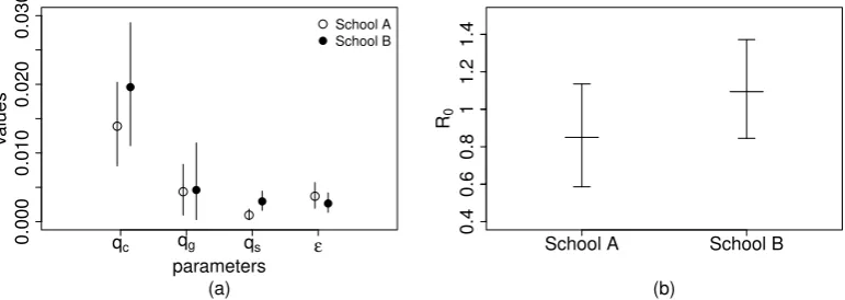
Parameters School A School B
mean of qc [95% CI] 1.39×10⁻² 1.96×10⁻²
[8.1×10⁻³−2.03×10⁻²] [1.11−2.89×10⁻²]
mean of qg [95% CI] 4.36×10⁻³ 4.61×10⁻³
[9.61×10⁻⁴−8.34×10⁻³] [2.98×10⁻⁴−1.15×10⁻²]
mean of qs [95% CI] 9.52×10⁻⁴ 2.96×10⁻³
[2.87×10⁻⁴−1.82×10⁻³] [1.64−4.45×10⁻³]
mean of ε [95% CI] 3.70×10⁻³ 2.65×10⁻³ [1.95−5.69×10⁻³] [1.37−4.2×10⁻³]
Table 4.4: Mean and 95%-credible intervals of the estimates for the infection
proba-bilities in schools A and B, when considering model CGS.
24 CHAPTER 4. PARAMETERS ESTIMATION
0.000
0.010
0.020
0.030
parameters
values
qc qg qs ε
School A School B
(a)
0.4
0.8
1.2
R0
School A School B
0.6
1
1.4
(b)
Figure 4.5: Estimated values of the transmission parameters for school A and B.
White and black dots represent the mean of the posterior distribution for
school A and school B respectively, bars represent 95%-credible intervals.
(b) Estimated values of the basic reproduction number R0 inside schools
A and B. Thick line and bars represent means and95%-credible intervals.
estimated class infection transmission probability is the highest of all settings. Grade transmission probability is estimated in both schools to be higher than school transmission; however the respective 95%-credible intervals overlap (just barely in school A, largely in school B).
As for comparisons between schools, estimates of class and grade transmission probability are similar, as is the probability of transmission from outside the school. On the other hand, estimates of school transmission probability differ between the two schools (95%-credible intervals barely overlap).
Using these estimates for transmission probabilities, we obtain from (4.1) the values of R0 shown in Figure 4.5b, with an average of 0.8503 in school A and
1.094 in school B. Note that (4.1) is based only on within-school transmission and does not include transmissions to household members or acquaintances; on the other hand, the estimates based on Figure 4.1 depend on all infected students, whatever their source of infection.
4.5
Model validation
4.5. MODEL VALIDATION 25
40
80
120
160
n
umber of inf
ectious individuals
School A School B
(a)
40
50
60
70
80
dur
ation of the epidemic (da
ys)
(b)
School A School B
Figure 4.6: The plot of the total number of infectious individuals (panel a) and the
duration of the epidemic (panel b) in 400 simulations. The black dot indicates the observed number of infectious individuals and the observed length of the epidemic in the two schools. Thick line and bars represent
means and 95%-credible intervals.
Chapter 5
Discussion
I
n this chapter we summarize and discuss the main results obtained by analysing the epidemic model introduced in Section 3.2 and we show how our results can be compared with the ones obtained in other works. We stress the limitations and introduce some possible improvements for this particular model such as explicit household transmission, school closure during weekends or asymptomatic cases.We estimated influenza transmission probabilities in a school setting, using the (incomplete) data collected through a retrospective survey conducted in December 2009 in two primary schools and we found that, in both schools, influenza was mainly transmitted within-class (Figure 4.5). Same- and different-grade transmission, as well as outside-school transmission, were all significantly lower than within-class transmission, with no significant differences between them (Figure 4.5).
We found that for both primary schools model CGS (that distinguishes within-class, same-grade and different-grade transmission) has the lowest DIC, i.e. is the favourite model overall. According to the DIC, models CGS and CS (that distinguishes within-class transmission from the general within-school transmission only) are equivalently good for school B, which reflects the similarity observed in the estimated same-grade and different-grade transmissions (Figure 4.5).
Similar results were obtained by Cauchemezet al.[16], where the transmission probability between students of the same class was five times greater than the transmission probability between students of the same grade and, in turn, this was five times higher than the transmission probability between students of different
28 CHAPTER 5. DISCUSSION
grades. The estimates we obtained are similar, with factors of 3-4 instead of 5, except for the grade-school ratio in school B, which is just above 1. These results are also consistent with the studies presented in [66, 67], where children used wearable sensors: in these studies it was found that children spent on average three times more time with children of the same class than with children of other classes. The fact that within-class transmission is estimated to be higher than within-school transmission can have implications on the design of school closure policies aimed at mitigating the spread of influenza, especially on evaluating the effectiveness of gradual closures (where single classes close first, then grades and finally the entire school) [66, 68, 69].
Another interesting result emerges from the comparison between the two schools involved in the study: while the estimates for within-class qc and
within-grade qg transmission probabilities are similar for the two schools, the estimate
for school-wide transmission qs is remarkably different, as 95%-credible intervals
barely overlap. This result can bear on the issue on whether infection transmission should depend on the density or the frequency of infectious individuals [70, 71]. In the model, we have assumed that transmission probability per individual is a constant. Alternatively, we could have adhered to the more usual assumption that transmission probability is inversely proportional to the number of individuals in that setting [72]; in case of school transmission, we should have used qs(A) =
c/ns(A) and qs(B) = c/ns(B). As ns(A)≈ 1.5ns(B), this results into qs(B) ≈
1.5qs(A). The mean estimated qs for school B is about 3 times the estimated
mean for school A, but 1.5 sits well inside the ratios of values in the 95%-credible intervals. Thus we can conclude that a frequency-dependent transmission probability is compatible with our findings, whereas density-dependent is not. It is remarkable that, while the estimates of transmission probabilities obtained in [16] are somewhat higher than ours, as for within-class and within-grade transmission, those of within-school transmission are similar to those of school A; this pattern appears to confirm that indeed larger school size (436 in the school studied in [16]) decreases per person transmission probability within school, although the social context may be very different, and there is no reason why contact patterns should be similar in Pennsylvania as in Italy. More studies comparing infection patterns in schools of different size but in a homogeneous social system, would be needed for such a conclusion.
29
the actual number of students in class each day; unfortunately such data was not available to us.
The estimates of the school R0 [School A mean and 95% CI 0.8503
(0.5859-1.1353) and School B 1.094 (0.845-1.372) ] lie in the low end of the spectrum of values estimated from influenza spread in schools [60]. In particular, our model provides estimates of R0 lower than 1 for school A, which highlights the
importance of outside transmission (with a likely strong role of households) in maintaining the school outbreak, consistently with the findings of [16].
As information on household cases was scarce, we had to rely on two simple models for outside transmission: either a constant probability ε or a probability proportional to influenza incidence in the population (variable ε). Concerning the latter, we could use only the weekly ILI incidence estimated through the surveillance system InfluNet; we used it at the Trento province level, that, on the one hand, is probably much larger than the territory where students of the two schools live, and, on the other hand, is smaller than the recommended aggregation level of sentinel data that makes them statistically significant. Despite these limitations, we deem that it yields the best available alternative to a constant probability of outside infection. The results of the comparison between the two model variants are not unequivocal: in School A model CGS with varying ε
yields a larger DIC than model CGS with a constant ε, while in School B the model with varying ε is much better than the model with constant ε.
An explanation for this contrasting result can be found in Figure 3.1. In School A, many scattered cases occur before infection takes off, while in School B almost no cases are recorded before the infection peak. Thus, to fit the pattern of infection observed in school A, the probability of infection from outside the school must have been non-negligible already from the second half of October, when overall ILI incidence was very low; if the probability of outside-school infection were proportional to ILI incidence,this would have forced it to become extremely large in November, which is hardly compatible with observed data. On the other hand, the infection trend school B is quite aligned with overall ILI incidence; thus, a model with outside-transmission proportional to overall incidence fits data very well. Clearly, this is an explanation for the statistical result, but does not clarify the reason (a localized epidemic in the community?) for the many scattered cases in School A before the epidemic start.
30 CHAPTER 5. DISCUSSION
times out of 50, it is found that 95%-credible intervals do not intersect, although, when it occurs,qc is always larger thanqs. On the other hand, whenqc is at least
3 times larger than qs (simulations 3-10 of Figure 4.3) a difference is picked up in
at least 85% of the cases. Furthermore, the algorithm produces correct estimates even in presence of missing data (we assumed 20% of those, similarly to actual data) and with errors in the reported dates (we assumed 30% of these), with the only visible effect of yielding somewhat wider credible intervals, relatively to the case of no missing data and no errors.
The choice ofγ = 0.1 for the probability that the effective (at school) infectious period lasts 2 days has been extrapolated from limited data presented in [54]) may appear questionable, and one may ask whetherγ could have been estimated as well from data. However, we show (Figure S1) that the algorithm we used is not capable on simulated data of estimating the probability γ of being infectious (at school) for 2 days, whatever is population size and the value of γ used for simulating data. Indeed, in most cases length of the infectious period and generation time are estimated from household studies or other cases where dates of infections can be independently established [70, 73]. As far as we know, the only exception is the study by White et al. [74], who were able to obtain an estimate of the serial interval from a detailed epidemiological curve. Our study shows that it is generally very difficult to do so.
Although the value of γ used in the study may be somewhat arbitrary, the main conclusions obtained on the differences between transmission probabilities in the different contexts and between two different schools do not depend on the exact value of γ; changing its value simply results in changing the numerical estimates of qc, qg and qs but not their relative features.
Similar identifiability problems led us to assume the simplified assumption that each student infected at school is infectious at school the following day, while it can be argued from the results in [54] that some will be infectious only in their second day after infection, and others will show symptoms before the first day and will be already kept home. Allowing for such possibilities would introduce other parameters that are difficult to estimate, without relevant effects on the main results.
There are several other aspects that we did not consider in our model, such as explicit household transmission, school closure during weekends or asymptomatic cases.
31
time in the school setting is short, weekends can break the transmission chain at school thus having an impact on the transmission pattern, as can be seen in [66, 67, 72, 75]. On the other hand, household and outside transmission is likely to increase during weekends, as often assumed in modelling studies [72,76]. Again, for the sake of simplicity, we preferred to avoid the introduction of parameters that may not be easily estimated, but in principle the model could be extended to distinguish between weekdays and weekends.
Our model assumes that all infections are symptomatic and lead to the same level of infectiousness. Indeed, using raw data, the estimate of children showing influenza symptoms is 52%. This value is comparable to the estimate of 56.9% infection rate for 2009H1N1v in primary-school children in Italy, that was derived from serological data [77]; thus, it seems likely that only a small number of children in those schools got infected with influenza without showing symptoms. Indeed, it is possible that the fraction of children of the schools considered in our study that got infected was much higher than the national average of 56.9%. Alternatively, it is possible that some of the children that reported symptoms were not actually infected with influenza virus, while others were infected but did not show symptoms. The lack of serological data prevents from a choice between different alternatives. Accordingly, we decided to use the most parsimonious alternative, namely to neglect asymptomatic infections.
Appendix A
Algorithm used to estimate
transmission probability in
schools for the 2009 H1N1
influenza pandemic in Italy
T
he available data are the knowledge on whether students have acquired infection or not, as well as the days of symptom onset (all this infor-mation will be named Z, where Zi is the day of symptom onset forindividuals i having acquired infection, while Zi = ∞ for the others). For the
moment, we neglect the problem of missing data.
We wish to obtain a posteriori distributions for the parameters qs, qA, qB and γ
(collectively named ϑ). As computing the likelihood of the data Z would be very complex, we include in the parameters to be estimated the dates Y of infection of the individuals that have become infected.
Then, through Bayes’ formula
fpost(ϑ, Y)∝P(Z|ϑ, Y)fprior(ϑ, Y) =
P(Z, Y|ϑ)
P(Y|ϑ) P(Y|ϑ)π(ϑ) =P(Z, Y|ϑ)π(ϑ). (A.1) where
P(Z, Y|ϑ) =Y
j,h
Tmax−1 Y
t=tmin
γI
j,h
2t+1(1−γ)(I
j,h
1t −I
j,h
2t+1)P(Sj,h
t+1|S
j,h
t , Itj,h, Itj, It). (A.2)
P(Stj,h+1|Stj,h, Itj,h, Itj, It) can be obtained from (3.2) , and the quantitiesStj,h, Itj,h, Itj, It
can all be easily computed from Y and Z.
34 APPENDIX A. THE ALGORITHM USED
The transition probabilitiespj,ht used in (3.2) can be written in a computationally more efficient way, by introducing the quantities qA and qB as
1−qA=
1−qc
1−qg
1−qB =
1−qg
1−qs
as
pj,ht = (1−qA)Itj,h(1−q
B)I
j t(1−q
s)It(1−ε) (A.3)
using the quantities
Itj =
nj X
l=1
Itjl (total number of infectious in gradej)
It =
5 X m=1 nm X l=1
Itml (total number of infectious in the school)
Missing data can be handled very easily in this framework: it is enough including in the vector of added parametersY the state (eventually infected or not) and, if so, the dates of infection and removal for all students whose information is missing.
The posterior distribution is estimated as the stationary distribution of the Markov chain resulting from Metropolis-Hastings algorithm [42, 56].
A.1
Parameters updating
To update the parameters we use a Single Component Metropolis-Hastings (see [56]) because, instead of updating all the parameters at once, it is often
computationally convenient to do that in different steps.
If we consider one of the infection rates qc, qg, qs, ε, the new state xis obtained in the following way
x= ye
ra
1−y+yera →
1 r → ∞
y r = 0 0 r → −∞
A.1. PARAMETERS UPDATING 35 So, by simple calculations, we obtain that,
q(y|x) = 1
y(1−y)√2πre − 1
2r2[log(x)+log(1−y)−log(y)+log(1−x)] 2
q(x|y) = 1
x(1−x)√2πre − 1
2r2[log(x)+log(1−y)−log(y)+log(1−x)]
2
and then qq((yx|x)
|y) is equal to
q(y|x)
q(x|y) =
x(1−x)
y(1−y).
Part II
Dynamics of Host-Parasitoid
Interactions and Coexistence of
Different Hosts


![arxiv: v3 [cs.cl] 3 Feb 2021](data:image/gif;base64,R0lGODlhAQABAIAAAP///wAAACH5BAEAAAAALAAAAAABAAEAAAICRAEAOw==)