Genetic algorithm to optimize two-echelon inventory control system for perishable goods in terms of active packaging Pages 103-114 Download PDF

(1)

* Corresponding author. Tel.: +

International Journal of Industrial Engineering Computations 3 (2012) 103–114

Contents lists available at GrowingScience

International Journal of Industrial Engineering Computations

homepage: www.GrowingScience.com/ijiec

Genetic algorithm to optimize two-echelon inventory control system for perishable goods in terms of active packaging

Narges Khanlarzadea*, Babak Yousefi Yeganeb and Isa Nakhaia

a_{Department of Industrial Engineering,, Faculty of Engineering, Tarbiat Modares University,Tehran, Iran} b_{Department of Industrial Engineering, Islamic Azad University, Malayer Branch, Malayer, Iran}

A R T I C L E I N F O A B S T R A C T

Article history: Received 1 July 2011 Received in revised form September, 30, 2011 Accepted 30 September 2011 Available online

12 October 2011

This paper considers an inventory control policy for a two-echelon inventory control system with one supplier-one buyer. We consider the case of deteriorating items which lead to shortage in supply chain. Therefore, it is necessary to decrease the deterioration rate by adding some specification to the packaging of these items that is known as active packaging. Although this packaging can reduce the deteriorating rate of products, but may be increases the cost of both supplier and buyer. Because of the complexity of the mathematical model, a genetic algorithm has been developed to determine the best policy of this inventory control system.

Keywords:

Supply chain

Two-echelon inventory control System active packaging Genetic algorithm

1. Introduction

There is an intense competition between various organization and institution across the world, and customers always expect products or services with high quality. Nowadays, Lack of monopoly in the market gives rise to the competition and leaves no room for any mistake in favor of suppliers and producers because it can lead to the loss of customers. Among different products, food and medicine have a great importance in the market, which can undergo different conditions for maintenance and thereby much attention should be paid to their packaging in order to keep the quality. Thus, the safety of these goods will be guaranteed, and the deterioration can be prevented so that the ideal attributes of food or medicine are preserved.

(2)

In this study, the impact of active packaging on the durability of products and the application of inventory control systems of perishable goods are taken into account in order to analyze the application of such methods in two-echelon supply chain in economic terms.

2. Packaging and perishable goods

Today, packaging has gained much momentum in the global market. Research indicates about 2% of GNP in the developed countries is attributed to packaging, in which 5% of the share for this industry goes for food packaging. The prediction indicates the packaging industry is increasing around the world.

New packaging systems have recently been developed to satisfy customer needs for quality, health, and durability of food and medicine. Furthermore, the delivery of products to the customers has experienced changes such as the concentration of the stores and the establishment of supermarkets, which delivered packages of food to the customers. Because of the distance between suppliers and consumers, a major revision on the role of packaging has been made in order to help better preservation of the products. Traditional packaging contributes to the distribution of products and can protect the products against physical condition such as light, oxygen, moisture, microbes, pressure and dust. Lack of accurate information on the durability and quality of products apart from erroneous measurement of the time period needed to maintain the products, are among the limitation of the systems. Some innovations including active packaging have developed to increase the efficiency, and to bridge the gaps in the industry. These novelties are to ensure the quality of products, determine the exact durability, and finally lessen the customers' complaints. In the following section, active packaging of food and medicine are briefly discussed within the boundary of the study.

The term "active packaging" was first used by Labuza (1996). The first active packaging was tin-plated steel used to make cans in the preserved food industry. Besides, mummified paper was, long before, used to inoculate sorbet into cheese. Nowadays, active packaging is widely used in US, Australia and Japan markets. The operation of active packaging, the conditions of preserved food with the aim of increasing the durability, improving safety or the sensory properties in the face of quality preservation are all affected by the method. This kind of packaging falls into two broad categories,

1. The absorbents of moisture, oxygen, carbon dioxide, ethylene, taste and smell; 2. The release of carbon, anti-microbe agent, and taste;

3. Literature review

Producers get their raw material from suppliers, transform them into finished goods and products, which in turn will be sold to distributers, and finally delivered to the final consumer or retailers. A multi-echelon inventory system is formed when a product travels all through these phases before it reaches the customer. Supply chain refers to a logistics network, which includes suppliers, distributers, raw material, work in process and the final product which all are circulated between different facilities and equipment. Researchers' interest has significantly grown in this field and many companies have a widely invested in this area.

(3)

& Wee, 2000). They considered an economic order policy of perishable goods for buyer and supplier as an integrated approach and developed a policy with the constant rate of production and demand. A mathematical model, based on both buyer's and seller's views, was developed with one buyer and one supplier and multiple deliveries for each order. They argued that a significant decrease was made in the costs by the integrated approach compared to the supplier's independent decision.

Wee et al. (2008) proposed an integrated supplier-buyer order policy for perishable goods. They developed the analysis made by Yang & Wee(2000) for one supplier-one buyer integrated production-inventory model with a deterioration rate corresponding to the inventory level. Aiming at developing a multi-echelon inventory model for perishable goods and obtaining the optimal common total cost through the integrity between buyer, producer and supplier, Rau et al. (2003) demonstrated that the least cost is attributable to the results obtained in the integration approach compared with independent decision approach. In this study, irrespective of consistent delivery, a lot-size model is developed for both the order and production of perishable goods, which has a fixed demand rate and an exponential deterioration function.

It is demonstrated that optimal supply chain is effective through integrated approach rather than independent approach. Huang (2002) proposed a model to obtain an optimal integrated policy of inventory-production and of supplier-buyer for perishable goods in JIT environment. Mahapatra and Maiti (2007) developed production-inventory models for perishable goods in a one supplier-one buyer system with a fixed demand production rate. Buyer's backlogging, if permitted, is a function of time and the model is formulated as the cost minimization problem via both integrated and disintegrated approaches. A genetic algorithm was used in the study to solve one or multi-objective production inventory problems.

Shah et al. (2008) developed a common buyer-supplier inventory system for perishable items with a salvage value. Based on a fixed deterioration rate, it was quantitatively demonstrated that the results acquired in the common approaches will have less cost than buyer's independent approach. Despite the decrease in common total cost, buyer's cost will rise due to the increase in orders. It is recommended that the supplier can postpone the payment, when permitted, in order to encourage the buyer to keep on the same approach so that more orders can be placed. In the study, the buyer-supplier common inventory system was developed for perishable goods with a salvage value.

Yu et al. (2008) proposed a mathematical model for a three echelon inventory system where integrate lower, middle and higher levels in supply chain. They hypothesized that deterioration is a function of the inventory available in the whole levels of chain. The problem of multi-echelon supply chain inventory was first resolved by simulated annealing algorithm, which always ensures the realization of global optimum.

(4)

4. Mathematical model

In the real-world, deterioration and decay in most of the products including food and medicine seems inevitable. In the former industries, due to the significant of delivering safe and sound products to the customer, producers and manufacturers have to meet numerous factors in order to determine the expiration date. They, finally, determine the time period permitted to maintain the products. However, almost always, a shorter time compared to the original specified period is recommended because of the safety standards. This shorter time is indicate on the package to prevent such repercussions as consumer poisoning, customer complaints and eventually lost sale as well as incurring high cost. Active packaging can directly lengthen the permitted maintenance period. Thereby the risk of errors in specifying the expiration date will be decreased; so in this case, the manufacturer does not have to indicate a shorter period on the packaging to meet the consumer safety criteria. Rather, the consumer is provided with more relevant information by having the original period indicated on the package.

The mathematical model, in two-echelon supply chain, is presented with activating variables along with inventory systems for perishable goods. The distinguishing features of proposed model compared to the former ones are as follows:

1. Adding activating variables of packaging to the mathematical model; 2. Determining lot size via cost analysis.

4.1 The variables in mathematical model

The problem under study is analyzed based on the following variables,

H: Planning horizon;

n: The number of replenishments for buyer during the planning horizon;

D: The demand rate that considered constant;

i

s: Is the time when shortages begin during the ith period , s_n H(i1,2,...,n1);

i

t : Is the time when the ith replenishment begin , t₀ 0(i1,2,...,n1); 1

 : The deterioration rate of the goods kept by buyer;

2

 : The deterioration rate of the goods kept by supplier;

3

 : The deterioration rate of the goods transported between supplier and buyer;

i

L: The time of production required to provide the buyer demand during period i;

bo

C : The cost of each replenishment for the buyer;

ss

C : The cost of each replenishment for the supplier;

bc

C : The cost of keeping the inventory incurred by buyer for each unit of goods during unit of time;

sc

C : The cost of keeping the inventory incurred by supplier for each unit of goods during unit of time;

bb

C : The cost of backlog incurred by buyer for each unit of goods during unit of time;

bd

C : The cost of each unit of goods deteriorated which is incurred by buyer;

sd

C : The cost of each deteriorated unit of goods incurred by supplier; )

(t

I_bi : The level of inventory for buyer during unit of time; )

(t

I_si : The level of inventory for supplier during unit of time; )

(t

(5)

:

P The production rate of supplier, where PD; :

i

RI The total inventory maintained by buyer during the i-th replenishment period )

,..., 2 , 1

(i n ; :

i

SI The total inventory maintained by supplier during the i-th replenishment period )

,..., 2 , 1

(i n ; :

i

RD The total number of deteriorated products for the buyer during the i-th replenishment period (i1,2,...,n);

: i

SD The total number of deteriorated products for the supplier during the i-th replenishment period (i1,2,...,n);

: i

RS The total shortage for the buyer during the interval



t_i,s_i



; :

 The rate of decrease in product's deterioration as a result of active packaging ( in other words refer to the extent of error which will decrease the deterioration rate via active packaging approaches, and will also lead to longer durability);

:

W The cost of active packaging ;

4.2. Research hypotheses

1. Just one buyer and one supplier areconsidered;

2. The buyer's shortage is allowed except during the last period where no shortage in the case of supplier is allowed;

3. The total cost of functions for both buyer and supplier during the entire period included )

, ,..., , , , ,

( ₁ ₁ ₂ ₂ _n_₁ _n_₁

b n s t s t s t

TC and TC_s(n,s₁,t₁,s₂,t₂,..., s_n_₁,t_n_₁), respectively;

4. The total cost is as following:

) , ,..., , , , , ( ) , ,..., , , , , ( )

, ,..., , , , ,

(n s₁ t₁ s₂ t₂ s_n_₁ t_n_₁ TC_b n s₁ t₁ s₂ t₂ s_n_₁ t_n_₁ TC_s n s₁ t₁ s₂ t₂ s_n_₁ t_n_₁ TC

4.3The proposed model

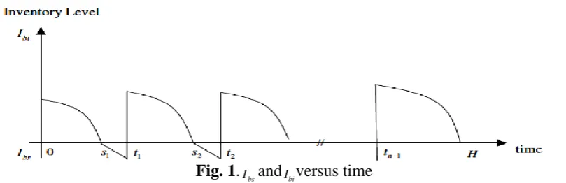
Fig. 1 depicts the inventory level and the buyer's shortage level in terms of time. The level of buyer's inventory will be depleted due to the combined effect of demand and deterioration.

Fig. 1.I_bsandI_biversus time

The instantaneous inventory level therefore is calculated as follow,

1 1

( )

( ) ( ) , , 1, 2,...,

bi

bi i i

dI t

I t D t t s i n

dt         

(1)

where the boundary condition Ibi(si)0is assumed. In addition, the shortage level for the buyer during

(6)

( )

, , 1, 2,..., 1 bs

i i

dI t

D s t t i n

dt       (2)

and the initial condition Ibs(si)0is assumed. Based on Eq. (1), Ibi(t) is formulated as follows,

1

1 1 ( ) ( )

( ) ( )

1 1

( ) ( 1), , 1, 2,...,

( )

i

s _s _t

t u

bi _t i i

D

I t e   e  D du e  t t s i n

 

 

  



     





(3)

According to equation (2), I_bs(t)is formulated as follow,

( ) ( ), , 1, 2,..., 1

bs i i i

I t D ts s  t t i n (4)

Therefore, the total inventory carried by the buyer during the interval



t_i_₁,s_i



is as follows,

1 1

( ) ( )

1 2

1 1

( ) ( 1) ( ), 1, 2,...,

( ) ( )

i i

s t

i bi i i

D D

RI I t dt e  s t i

    

 



     

 



₍₅₎

In particular, in the final period:

1 1

1

( ) ( )

1 2

1 1

( ) ( 1) ( )

( ) ( )

n n

H

H t

n bi n

t

D D

RI I t dt e  H t

    



 



    

 



(6)

the interval

 

s_i,t_i , the total amount of shortage for the buyer is as follows:

2

( ) ( ) , 1, 2,..., 1 2

i

t

i _s bs i i

D

RS 



I t dt t s i n (7)

For the buyer, the total number of goods deteriorated in the ith replenishment period is as following:

1 1

1

( ) ( )

1 1

1

( ) ( 1) ( ), 1, 2,... 1

( )

i

i i i

s

s t

i bi i _t i i

D

RD I t D du e  D s t i n

  



 

       





(8)

and, in particular, for the final period,

1 1

1

( ) ( )

1 1

1

( ) ( 1) ( )

( )

n n

H

H t

n bi n _t n

D

RD I t D du e  D H t

  



 

     





(9)

Therefore, the total cost for the buyer over the planning horizon is as follows,

1

1 1 2 2 1 1

1 1 1

( , , , , ,..., , )

n n n

b n n bo bc i bd i bb i

i i i

TC n s t s t s t nC C RI C RD C RS



 

  

 











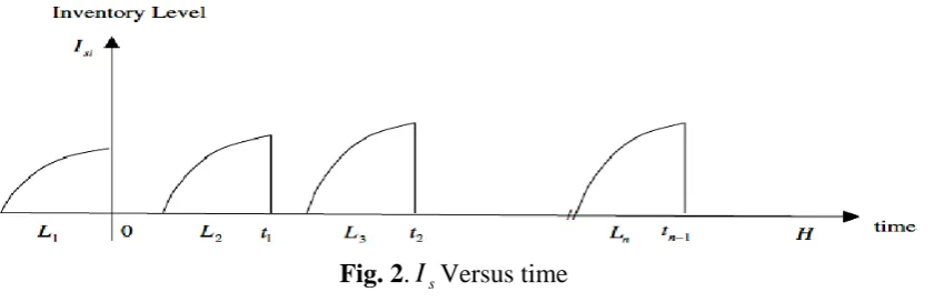
₍₁₀₎

(7)

Fig. 2.I_sVersus time

Therefore, the supplier's temporal inventory level is as follow,

2 1 1

( )

( ) ( ) , , 1, 2,...,

si

si i i i

dI t

I t P t L t t i n

dt           (11)

where the boundary condition I_si(t_i_₁L_i)0 is valid. Based on Eq. (11), I_si(t) is formulated as follow, 1 2 1 2 2 1 ( )( ) ( ) ( ) 1 1 2

( ) (1 ), , 1, 2,...,

( )

i

i i i i

t _t _{L t}

t u

si _t _L i i i

P

I t e   e  P du e  t L t t i n

                     



(12)

where L_i is calculated via the following two equations:

) ( ) ( )) ( 1

(  ₃ I_si t₀ I_bi t₀ 1 ,..., 2 , 1 ), ( ) ( ) ( )) ( 1

(  3  Isi ti Ibi ti Ibs ti i n

Thus, the result is the follow,

1 1

( ) 2

1

2 1 3

( )

1

[1 ( 1)]

( ) ( ) (1 ( ))

s

D

L Ln e

P                     (13) 1 1 ( ) ( ) 2

1 1 1

2 1 3

( )

1

[1 [( 1) ( ) ( )]], 2, 3,...,

( ) ( ) (1 ( ))

i i

s t

i i i

D

L Ln e t s i n

P     _{ }                         (14)

Consequently, the total number of inventory carried by the supplier during the production interval

t0  Li,t0 would be as follow,

1

0

1 2 1 1

2

( ) [ ( ) [1 ( )]]

( )

si L

P

SI I t dt s Ln s

 



      





(15)

where ₍ ₁₎

)) ( 1 )( ( ) ( )

( (1 )1

3 1

2

1 _ _ _ 

 

  s

e P D

s  

   



 _{. Integrated during the production period}

_

_

i i

i L t

t1 , where

n

i 2,3,..., , the total inventory maintained by the supplier would be as follow,

1

1 1 1 1

2 2

( ) [ ( , , ) [1 ( , , )]], 2, 3,...,

( )

i

i i

t

i _t _L si i i i i i i

P

SI I t dt s t s Ln s t s i n

                



(16)

where _[( ₁₎ ₍ ₎₍ _)]

)) ( 1 ( ) ( ) ( ) , ,

( 1 1 1

) ( ) ( 3 1 2 1 1 1      _ _ _         i i t s i i

i e t s

P D s

t

s i i  

   



   _{. In the first replenishment}

(8)

TC

2 

0 )

( 2

) , ( 2 1

2

* 2 * 1

 

  

t t

P

1 1

( )

1 1 0 1

2 1

( ) [1 ( )] ( 1)

( ) ( )

s bi

P D

SD PL I t Ln s e 

    

       

 

(17)

Thereby, the total deteriorated goods in the ith replenishment period for the supplier are as follow,

1

( ) ( )

1 1 1 1 1 1

2 1

( ) ( ) [1 ( , , )] [ 1] ( ), 1,...,

( ) ( )

i i

s t

i i bi i bs i i i i i i

P D

SD PL I t I t Ln s t s e  D t s i n

     

     

           

 

(18)

Thus, the total cost for the supplier during planning horizon H is as follow,

1 1 2 2 1 1

1 1

( , , , , ,..., , ) ( )

n n

s n n ss sc i sd i

i i

TC n s t s t s_ t _ n C W C SI C SD

 

  







(19)

As a result, the total common cost of the entire inventory system is as follows,

1 1 2 2 1 1 1 1 2 2 1 1 1 1 2 2 1 1

( , , , , ,..., _n , _n ) _b( , , , , ,..., _n , _n ) _s( , , , , ,..., _n , _n )

TC n s t s t s _ t _ TC n s t s t s _ t _ TC n s t s t s_ t _ (20)

The objective of this study is to determinet_iands_i, so that the total cost of inventory system is minimized. For a fixed n, the necessary condition for TC to be the minimum is:

     

 

  

 

  

; 1 ,... 2 , 1 , 0

n i

t TC

n i

s TC

i i

We assume that the deteriorating rate for supplier, buyer is same; also we assume that the transportation of the goods between supplier and buyer has the same effect on deterioration of products, in other words we assign a similar Lambda for supplier, buyer and transportation between them.

Theorem1.Hessian matrix is positive definite if nvalues are positive and cardinal.

It means that the target function has an absolute minimal point.

Proof. Due to the complexity and multiplicity of the model variables, the mathematical problem was simplified using Mathematica software V.6., the results show that Hessian matrix is positive definite, meaning:

) (

) det(

) , ( 2 2 2

) , ( 2 1 2

* 2 * 1 *

2 *

1t t t

t t

P

t P H

   

 

5. The proposed GA method

(9)

5.1. Chromosome

One of the most important factors for successful implementation of MA is designing a more suitable chromosomal structure. In this paper, the solution consists of a matrix with one row and ݇ columns. In each column, a number with four digits is placed. Fig. 3 shows the proposed chromosomal structure of the paper.

t3 t2

t1 S4

S3 S2

S1

Fig. 3.Chromosomal structure proposed for n=4

5.2 Initial population

As noted previously, the initial population is generated randomly. Although random generation covers almost all of the search space, a high-quality solution, obtained from another heuristic technique as an initial population, might help GA to find better solution.

5.3Evaluation

A fitness function is required to evaluate the chromosomes of each generation. In this study, like most GA application the total cost function of the model is considered as fitness function.

5.4 Selection

At this stage, parents are selected using one of the most popular selection methods called roulette-wheel. In this method, the parents are chosen based on the probability distribution of their fitness value and copied into the mating pool. Thus, the chance of selecting the best individuals becomes higher.

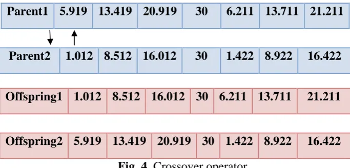
5.5Crossover

After parent selections, several pairs of chromosomes are selected randomly from mating pool by predetermined crossover rate and are mixed to produce offspring. In a crossover operation, some of genes in the first selected parent are replaced with the corresponding genes in the other parent. In this paper we define a new crossover operation that only changed the place of the genes that illustrate si

or ti, after applying this operation, other genes are completed from the changed genes (see Fig. 4).

21.211 13.711

6.211 30

20.919 13.419

5.919 Parent1

16.422 8.922

1.422 30

16.012 8.512

1.012 Parent2

21.211 13.711

6.211 30

16.012 8.512

1.012 Offspring1

16.422 8.922

1.422 30

20.919 13.419

5.919 Offspring2

(10)

5.6 Mutation

To prevent all solutions in population from falling into a local optimum, mutation takes place after a crossover is performed. In order to obtain a new offspring by using mutation operator in this paper mutation changed s1 or t1 in a specified chromosome. Mutation operator is shown in Fig. 5.

21.211 13.711

6.211 30

20.919 13.419

5.919

22.325

14.825 7.325

30 20.919 13.419

5.919

16.422

8.922 1.422

30 16.012 8.512

1.012

16.422

8.922 1.422

30 15.786 8.286

0.786

Fig. 5. Mutation operator

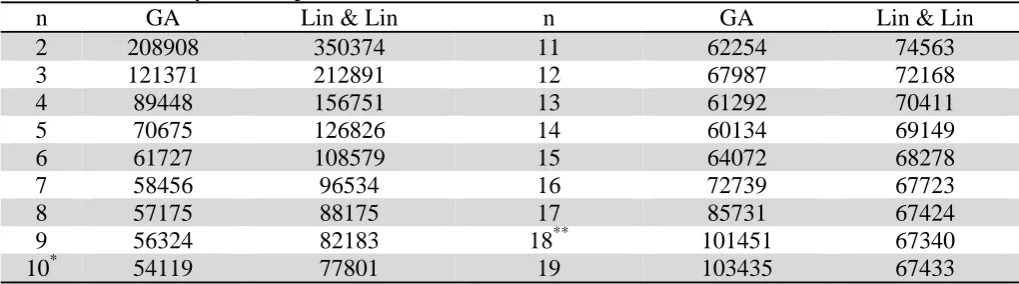
6. Computational methods

In this section, we examine the results of solving the model. To solve the mathematical model, a genetic algorithm was proposed and coded in VB6. To verify the effectiveness of the proposed GA, presented problem by Lin and Lin (2007) was resolved and obtained results are shown in Table 1. Compared with the results of Lin & Lin (2007), the effectiveness of our proposed algorithm is verified (the number of replenishments and total cost of the supply chain is considerably reduced). In developing phase, the parameters of active packaging are added to the model and the results are compared with state of ordinary packaging. It is noteworthy that different deterioration rates for each level of the supply chain were defined, for each of these values the mathematical model was solved separately. (It is necessary to note that the calculation results were given only if the values would

have led to the feasible solution). All parameters are the same as Lin & Lin (2007) and the value of  and W are as follows:



(0.001,0.01),(0.002,0.02),(0.004,0.03),(0.006,0.04),(0.008,0.05)



) ,

(



w 

Table1

Obtained results by GA compared with the results of Lin & Lin (2007)

Lin & Lin

GA n

Lin & Lin

GA

n

74563 62254

11 350374

208908 2

72168 67987

12 212891

121371 3

70411 61292

13 156751

89448 4

69149 60134

14 126826

70675 5

68278 64072

15 108579

61727 6

67723 72739

16 96534

58456 7

67424 85731

17 88175

57175 8

67340 101451

18** 82183

56324 9

67433 103435

19 77801

54119 10*

*Number of replenishment obtained by G

(11)

7. Conclusions

The study investigated a two-echelon inventory control system for perishable goods. In the mathematical models an additional hypothesis was inserted which involved studying the economy of using new packaging systems such as active packaging in inventory control systems for non-perishable goods. The results obtained through solving the problem confirm the economical hypothesis. Since usually the orders are practically in the front of fixed lots, the best lot size was selected through analyzing the cost in the proximity of the optimal point so that compared to the optimal cost; the lowest cost increase is made.

Table2

Determining the number of replenishment in terms of active packaging parameter

n (withoutandW ) n

(with andW ) TC

(withoutandW ) TC (with andW )

Stat TC  w 3  2  1  3 2

1  

   10 9 51837 42626 0.006 0.04 0.01 0.01 0.01 8 9 56381 51245 0.006 0.04 0.02 0.02 0.02 8 7 54105 52970 0.008 0.05 0.03 0.03 0.03 8 7 48973 50607 0.001 0.01 0.04 0.04 0.04 8 7 38365 42116 0.001 0.01 0.05 0.05 0.05 10 9 25490 27388 0.001 0.01 0.06 0.06 0.06 3 2

1  

(12)

Acknowledgment

The authors would like to thank the anonymous referees for constructive comments on earlier version of this paper.

References

Balkhi, Z.T., (1999). On the global optimal solution to an integrated inventory system with general time-varying demand,production and deterioration rates. European Journal of Operational and Research, 114, 29-37.

Huang, C.K., (2002). An integrated vendor-buyer co-operative inventory model for items with imperfect quality. Production Planning & Control, 13(4), 355-361.

Labuza, T.P.,(1996). An introduction to active packaging for foods. Food Technology, 50, 68-71. Lin, C. & Lin, Y., (2007). A cooperative inventory policy with deteriorating items for a two -

echelone model. European Journal of Operational Research , 178, 92-111.

Mahapatra, N.K., Das, K. & Maiti, M., (2007). Production-inventory policy for a deteriorating item with a single vendor-buyer system. Optim Eng, 8, 431-448.

Rau, H., Wu, M.Y. & Wee, H.M., (2003). Integrated inventory model for deteriorating items under a multi-echelon supply chain environment. International Journal of Production Economics, 86, 155-168.

Shah, N.H., Gor, A.S. & Wee, H.M., (2008). Optimal joint vendor-buyer inventory strategy for deteriorating items with salvage value.

Wee, H., Chung, C.J. & Yang, P.C., (2008). An integrated vendor - buyer deteriorating item ordering policy. Proceedings of the seventh International Conference on Machine Learning and Cybernetics,Kunming , 12-15.

Yang, P.C. & Wee, H.M., (2002). A single-vendor and multi-buyers production-inventory policy for a deteriorating item. European Journal of Operational Research, 143, 570-581.

Yang, P.C. & Wee, H.M., (2000). Economic order policy of deteriorated item for vendor and buyer: An integrated approach. Production Planning and Control, 11,474-480.

Yu, J.C.P., Wee, H.M. & Wang, K.J., (2008). An integrated three-echelon supply chain model for deteriorating items via simulated annealing method. Proceeding of the Seventh International