Differential search algorithm-based parametric optimization of electrochemical micromachining processes Pages 41-54 Download PDF

(1)

International Journal of Industrial Engineering Computations 5 (2014) 41–54

Contents lists available at GrowingScience

International Journal of Industrial Engineering Computations

homepage: www.GrowingScience.com/ijiec

Differential search algorithm-based parametric optimization of electrochemical micromachining processes

Debkalpa Goswami and Shankar Chakraborty*

Department of Production Engineering, Jadavpur University, Kolkata - 700 032, West Bengal, India

C H R O N I C L E A B S T R A C T

Article history: Received June 2 2013

Received in revised format August 15 2013

Accepted August 15 2013 Available online August 19 2013

Electrochemical micromachining (EMM) appears to be a very promising micromachining process for having higher machining rate, better precision and control, reliability, flexibility, environmental acceptability, and capability of machining a wide range of materials. It permits machining of chemically resistant materials, like titanium, copper alloys, super alloys and stainless steel to be used in biomedical, electronic, micro-electromechanical system and nano-electromechanical system applications. Therefore, the optimal use of an EMM process for achieving enhanced machining rate and improved profile accuracy demands selection of its various machining parameters. Various optimization tools, primarily Derringer’s desirability function approach have been employed by the past researchers for deriving the best parametric settings of EMM processes, which inherently lead to sub-optimal or near optimal solutions. In this paper, an attempt is made to apply an almost new optimization tool, i.e. differential search algorithm (DSA) for parametric optimization of three EMM processes. A comparative study of optimization performance between DSA, genetic algorithm and desirability function approach proves the wide acceptability of DSA as a global optimization tool.

Electrochemical micromachining process

Differential search algorithm Process parameter Response

1. Introduction

(2)

the tool-workpiece interface etc. Sometimes, it is also difficult to machine complex and intricate shapes employing the conventional processes. Since there will be continuous demand for miniaturization for efficient space utilization with better quality of products, micromachining technology will become still more important in the future (Bhattacharyya et al., 2004).

When electrochemical machining (ECM) process is used in the micron range of application, it is called electrochemical micromachining (EMM) process. EMM is a very promising micromachining technology due to its various inherent advantages, like high material removal rate (MRR), better precision and control, reliability, flexibility, environmental acceptability and green manufacturing. It is widely used to machine hard materials at a high MRR, without affecting the tensile strength of the workpiece material and its other physical properties, while ensuring a low surface roughness. It also permits machining of chemically resistant materials like, titanium, copper alloys, super alloys and stainless steel, which are now widely used in biomedical, electronic, micro-electromechanical system

(MEMS) and nano-electromechanical system (NEMS) applications. EMM process could be used as one

the best micromachining techniques for machining electrically conducting, tough and difficult to machine materials with appropriate combination of machining parameters. The desired quality of the workpiece in EMM process can only be generated through combinational control of its various process

parameters. Therefore, the optimal use of EMM process for achieving higher MRR, improved profile

accuracy and surface quality demands proper control of its process parameters. However, to exploit the full potential of EMM process, research is still needed to improve the machining accuracy by controlling its different machining parameters and determining the optimal parametric combination. An

excellent review on the machining mechanism of EMM process can be found in Bhattacharyya et al.

(2004) and Cao et al. (2012).

2. Survey of past research

Bhattacharyya et al. (2001) designed and developed an EMM setup comprising of various mechanical machining components, electrical system, an electrolyte flow system and a microprocessor-controlled end-gap controlling system. Bhattacharyya et al. (2002) developed an EMM system setup for performing basic and fundamental research in the area of EMM, fulfilling the objectives of

micromachining. Bhattacharyya and Munda (2003a) investigated the influence of machining voltage,

electrolyte concentration, pulse-on time and frequency of pulsed power supply on MRR and accuracy for effective utilization of an ECM system for micromachining operation. Bhattacharyya and Munda

(2003b) developed an EMM setup to meet the micromachining requirements, and indicated the most

effective zone of predominant process parameters, such as machining voltage and electrolyte concentration for providing the appreciable amount of MRR with less overcut. Bhattacharyya et al. (2005) studied the influence of various EMM process parameters, like machining voltage, electrolyte concentration, pulse period and frequency on MRR, accuracy and surface finish in microscopic domain. Kurita et al. (2006) determined the optimal values of machining voltage, machining pulse length, amplitude of the electrode for flushing out contamination and electrolyte concentration, and carried out three-dimensional shape micromachining at the derived optimal conditions. Bhattacharyya et al. (2007) carried out experiments to determine the optimal values of different EMM process parameters, such as micro-tool vibration frequency, amplitude and electrolyte concentration for producing micro-holes with higher accuracy and appreciable amount of MRR. Using response surface methodology (RSM), Munda et al. (2007) correlated the interactive and higher-order influences of various machining parameters on the combined effect of micro-spark and stray-current machining in an

EMM process. Munda and Bhattacharyya (2008) developed a mathematical model for correlating the

interactive and higher-order influences of various EMM process parameters, i.e. machining voltage pulse on/off ratio, machining voltage, electrolyte concentration, voltage frequency and tool vibration

frequency on MRR and radial overcut (ROC). Munda et al. (2010) developed mathematical models for

(3)

setting to produce better quality machined products at a higher rate. Li and Niu (2010) carried out experiments to investigate the influence of some EMM process parameters, such as pulse frequency, feed rate of tool, machining voltage and ultrasonic frequency on the machining accuracy of micro-holes. Malapati and Bhattacharyya (2011) considered five EMM process parameters, i.e. pulse frequency, machining voltage, duty ratio, electrolyte concentration and micro-tool feed rate, and studied their influences on two important responses, i.e. MRR and machining accuracy, during micro-channel generation. The optimal values of those process parameters were also found out employing desirability function approach. Malapati et al. (2011) studied the effect of various EMM process parameters, i.e. machining voltage, electrolyte concentration, frequency pulse period and duty factor on MRR and machining accuracy to meet the micromachining requirements. Malapati et al. (2012) investigated the influence of different process parameters on micromachining criterion using Taguchi method of robust design, and developed second order regression models to search for the best parametric combination to achieve the desired micromachining characteristics. Mithu et al. (2012) fabricated micro nozzles and micro pockets by EMM process. Rao and Patel (2012) introduced the elitism concept in teaching-learning-based optimization algorithm and investigated the effects of common controlling parameters, like population size and number of generations on the performance of that algorithm. Its optimization performance was also compared with that of other well known evolutionary algorithms. Thanigaivelan and Arunachalam (2013) optimized the process parameters for EMM operation of 304 stainless steel using grey relational analysis. Machining voltage, pulse on-time, electrolyte concentration and tool tip shapes were selected as the typical process parameters, and machining rate and overcut were the responses.

The past researchers have already applied various optimization tools and techniques, mainly Taguchi method and Derringer’s desirability function approach for finding out the optimal settings of EMM process parameters. But, those adopted approaches have several inherent limitations (especially generation of near optimal or sub-optimal solutions and high computational time) which compel the authors to explore the feasibility and acceptability of an almost unexplored optimization tool, i.e. differential search algorithm (DSA) for parametric optimization of EMM processes.

3. Differential search algorithm

The sustainability and efficiency of food sources available in nature (pastures, water supplies etc.) typically vary with the periodicity of seasonal changes. Thus, it is the characteristic of many species (eusocial, subsocial or presocial) to show seasonal migratory behavior to move to a more thriving

habitat (Krebs and Davies, 1997). The migrating species of living beings constitute a superorganism,

containing a large number of individuals.

There are a number of stochastic computational intelligence algorithms that model the behavior of superorganisms. Some of the most popular algorithms in this category include particle swarm optimization (PSO), cuckoo search (CS), artificial bee colony (ABC) algorithm, ant colony optimization (ACO) etc. The differential search algorithm (DSA) is the latest addition to this group.

Movement of a superorganism can be described by a Brownian-like random walk model (Trianni et al.,

2011). In DSA, it is assumed that a population made up of random solutions of the respective problem

corresponds to an artificial superorganism migration (Civicioglu, 2012). This superorganism tends to

migrate to a global minimum of the problem. In the course of this migration, the artificial superorganism tests whether some randomly selected positions are temporarily suitable for stop-over.

If it is so, members of the superorganism that made this discovery immediately settle at this discovered

position and continue their migration from here on.

(4)

Pseudo code: Differential search algorithm

Require:

N: Size of the population, where i = {1,2,3,…,N}

D: Dimension of the problem

G: Number of maximum generation

1: Superorganism = initialize(), where Superorganism =[ArtificialOrganismi] 2: yi = Evaluate(ArtificialOrganismi)

3: for cycle = 1: Gdo

4: donor = SuperorganismRandom_Shuffling(i)

5: Scalerandg[2rand1] ( rand2rand3)

6: StopoverSiteSuperorganismScale donor( Superorganism)

7: p10.3rand4 and p20.3rand5

8: ifrand6 < rand7then

9: ifrand8 < p1then

10: r = rand(N,D)

11: forCounter1 = 1: Ndo

12: r Counter( 1,:)r Counter( 1,:)rand₉

13: end for

14: else

15: r = ones(N,D)

17: r Counter( 2,randi D( ))r Counter( 2,randi D( ))rand₁₀

18: end for

19: end if

20: else

21: r = ones(N,D)

23: drandi D( ,1,p2rand D )

24: forCounter4 = 1:size d( ) do

25: r Counter d Counter( 3, ( 4))0

26: end for

27: end for

28: end if

29: individualsI J, rI J, 0 |Ii J, [1, ]D

30: StopoverSite individuals( I J, ) :Superorganism individuals( I J, )

31: if StopoverSitei j, lowi j, or StopverSitei j, upi j, then

32: StopoverSitei j, :rand(upjlowj)lowj

33: end if

34: yStopoverSite i; evaluate StopoverSite( i)

35: _; ; ; ;

;

: StopoverSite i StopoverSite i Superorganism i

Superorganism i

y y y

y

y else

 

  

36: i: i StopoverSite i; Superorganism i;

i

StopoverSite y y

ArtificialOrganism

ArtificialOrganism else

 

   37: end for

(5)

, ( )

i j j j j

x rand up low low (1)

Subsequently, the artificial organisms are defined by Xi = [xi,j] and the superorganism made up of these artificial organisms is denoted by Superorganismg= [Xi]. The mechanism of finding a stop-over site involves implementation of the Brownian-like random walk model (Trianni et al., 2011). The randomly selected individuals of the artificial organisms move towards the targets of donor =[XRandom_Shuffling(i)] in

order to discover these stop-over sites, which are pivotal for a successful migration. The magnitude of

the change in positions of the members of the artificial organisms is governed by the Scale factor. The

value of Scale is determined using a gamma random number generator (randg), which in turn, is

controlled by a uniform random number generator (rand). This coding structure (refer to line 5 of

pseudo code) allows the artificial superorganism to radically change direction within the habitat.

The expression for a stop-over site position is given by the following equation:

( )

StopoverSiteSuperorganismScale donorSuperorganism (2)

The members which participate in the search process for stop-over sites are determined by a stochastic scheme (lines 8-28 of pseudo code). Since this process is completely random, there is a probability that an element of the stop-over site is beyond the limits of the habitat (i.e. search space). To make the code foolproof against this situation, a suitable check is hence devised (lines 31-33 of pseudo-code).

If a stop-over site is more thriving than the sources owned by the artificial organism, the artificial organism moves to the newly discovered stop-over site. While the artificial organisms change site, the superorganism continues its migration towards the global optimum.

Two unique characteristics of DSA make it a successful search tool for solution of multi-modal functions. Firstly, DSA may simultaneously use more than one individual; and secondly, this algorithm

has no inclination to go towards the so-called best possible solution of the problem. These features are

unlike the other existing algorithms, like PSO, ABC etc. These traits are also evident from the nature of the scatter plots generated by DSA (given in sub-section 4.1 of this paper). The scatter diagrams generated by algorithms, like ABC and PSO clearly show a clustering of navigated data points near the optima (Samanta & Chakraborty, 2011). But in case of DSA, such a behavior is not to be observed (refer to scatter diagrams given in sub-section 4.1 of this paper).

The DSA has only two control parameters, p1 and p2 (line 7 of pseudo code). Civicioglu (2012)

conducted detailed tests to determine the most appropriate values for these two control parameters, and concluded that this algorithm is not much sensitive to the values of p1 and p2. The straightforward algorithmic structure of DSA allows for its easy application in practical engineering problems of interest.

4. Illustrative examples

(6)

4.1 Example 1

Malapati and Bhattacharyya (2011) developed an EMM setup to study the influence of various process parameters, like pulse frequency, machining voltage, duty ratio, electrolyte concentration and tool feed rate on MRR, width-overcut (WOC), length-overcut (LOC) and linearity during micro-channel generation. In order to develop the relationships between the considered five EMM process

parameters and responses, 32 experiments were conducted on bare copper plates

(15mm×10mm×0.15mm) using a central composite half factorial second-order rotatable design plan. Each of the EMM process parameters was set at five different levels, as given in Table 1. Among the considered responses, MRR is the ratio of difference in weights (final weight − initial weight) to the machining time, WOC is the excess dimensional machining across the micro-channel, LOC is the excess dimensional machining along the micro-channel and linearity is defined as the uniformity of width along the length of the generated micro-channel. Using the experimental data and with the help of MINITAB software, Malapati and Bhattacharyya (2011) developed four RSM-based equations for the considered responses, as given by Eqs. (3-6), to explore the interactive and higher-order effects of various EMM process parameters on the responses.

Table 1

EMM process parameters along with their levels (Malapati and Bhattacharyya, 2011)

Parameter Unit Levels

−2 −1 0 +1 +2

Pulse frequency (x1) kHz 40 50 60 70 80

Machining voltage (x2) V 7 8 9 10 11

Duty ratio (x3) % 30 40 50 60 70

Electrolyte concentration (x4) g/l 50 60 70 80 90 Micro-tool feed rate (x5) μm/sec 150 175 200 225 250

YMRR = 2.59446 + 0.237004x2 + 0.426029x3 + 0.340938x4 − 0.385790x12+ 0.295540x22 −

0.299427x32 + 0.224331x1x5 + 0.327156x2x3 − 0.243256x2x4

(3)

YWOC = 0.124856 + 0.0288208x4 + 0.0270208x5 − 0.0173807x32 + 0.0140443x52 +

0.0203563x1x4 − 0.0257063x1x5 − 0.0209313x2x3

(4)

YLOC = 0.403467 + 0.0526542x2 + 0.0604563x1x2 + 0.0457563x1x3 + 0.0344187x1x4 −

0.166544x2x4 − 0.0554562x2x5 + 0.0495813x3x4 + 0.0413687x3x5 + 0.0534565x4x5

(5)

YLinearity = 0.0721852 + 0.00868750x1 + 0.0112125x2 + 0.0171458x4 − 0.0128688x1x3 +

0.0151188x1x4 + 0.00841875x2x4 − 0.0116062x2x5 − 0.00749375x4x5

(6)

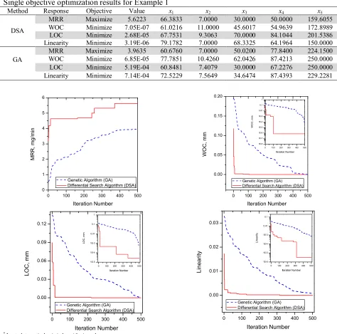
Single objective optimization

In single objective optimization, all the four responses of the considered EMM process, i.e. MRR, WOC, LOC and linearity, are separately optimized using DSA. Among these responses, MRR needs to be maximized and the remaining three responses are to be minimized. For all these single objective optimization problems, the constraints are set as 40 ≤ x1 ≤ 80, 7 ≤ x2 ≤ 11, 30 ≤ x3 ≤ 70, 50 ≤ x4 ≤ 90 and

150 ≤ x5 ≤ 250. In Table 2, the results of single objective optimization of the responses are presented

(7)

the values of all the considered responses. While solving the above-mentioned single objective optimization problems on an Intel® Core™ i5-2450M CPU @ 2.50 GHz with 4.00 GB RAM computing platform, the average computational time taken by DSA is 8.11sec, whereas, GA takes an

average of 12.41 sec to solve those problems.Fig. 1compares the convergence of DSA and GA for all

the four responses and it is clear that DSA is quite faster than GA in achieving the optimal values of the

responses. AsMalapati and Bhattacharyya (2011) did not perform any single objective optimization of

the responses, the results of DSA cannot be compared with theirs.

Table 2

Single objective optimization results for Example 1

Method Response Objective Value x1 x2 x3 x4 x5

DSA

MRR Maximize 5.6223 66.3833 7.0000 30.0000 50.0000 159.6055 WOC Minimize 7.05E-07 61.0216 11.0000 45.6017 54.9639 172.8989 LOC Minimize 2.68E-05 67.7531 9.3063 70.0000 84.1044 201.5386 Linearity Minimize 3.19E-06 79.1782 7.0000 68.3325 64.1964 150.0000

GA

MRR Maximize 3.9635 60.6760 7.0000 50.0200 77.8400 224.1500 WOC Minimize 6.85E-05 77.7851 10.4260 62.0426 87.4213 250.0000 LOC Minimize 5.19E-04 60.8481 7.4079 30.0000 67.2276 250.0000 Linearity Minimize 7.14E-04 72.5229 7.5649 34.6474 87.4393 229.2281

0 100 200 300 400 500

0 1 2 3 4 5 6 MR R, mg/min Iteration Number Genetic Algorithm (GA) Differential Search Algorithm (DSA)

0 100 200 300 400 500 0.00

0.05 0.10 0.15 0.20

0 100 200 300 400 500

1E-8 1E-7 1E-6 1E-5 1E-4 1E-3 0.01 0.1 1 WO C, m m Iteration Number WOC , mm Iteration Number

Genetic Algorithm (GA) Differential Search Algorithm (DSA)

0 100 200 300 400 500 0.00

0.03 0.06 0.09 0.12

0 100 200 300 400 500

1E-5 1E-4 1E-3 0.01 0.1 1 L OC , mm Iteration Number LOC, m m Iteration Number

0 100 200 300 400 500

0.00 0.01 0.02 0.03

0 100 200 300 400 500

1E-6 1E-5 1E-4 1E-3 0.01 0.1 L in ea ri ty Iteration Number Lineari ty Iteration Number

*

Inset plot: vertical axis in logarithmic scale

Fig. 1. Convergence diagrams of DSA and GA for Example 1

(8)

Increase in duty ratio would also increase the dissolution rate, and these products cannot be efficiently flushed out, once the duty ratio crosses the limit of 50%. Up to 50% duty ratio, the on-time is lower than off-time of pulse period, hence, the dissolved products can be flushed out easily. Beyond 50% duty ratio, the dissolved products may pile up in the machining zone, disrupting the dissolution process and reducing the MRR. It was also found out that MRR would increase with electrolyte concentration. At higher concentration, more ions would be associated with machining, thus increasing the current density that would lead to higher MRR. Due to increase in machining voltage, machining current would also increase, leading to increase in current density which causes higher MRR. It was also observed that the value of MRR would increase non-linearly with increasing values of machining voltage. At higher machining voltage, ions associated with the machining process would be more, which may have an impact in enhancing the value of MRR.

40 50 60 70 80

0 1 2 3 4 5 6

Differential Search Algorithm Malapati and Bhattacharyya (2011)

M

RR, mg

/m

in

Pulse Frequency, kHz

7 8 9 10 11

0 1 2 3 4 5 6

MR

R, mg/m

in

Machining Voltage, V 30 40 50 60 70

0 1 2 3 4 5 6

MRR, mg

/min

Duty Ratio, %

50 60 70 80 90

0 1 2 3 4 5 6

M

RR

, m

g/

min

Electrolyte Concentration, g/l

160 180 200 220 240

0 1 2 3 4 5 6

MRR

, m

g/min

Micro-tool feed rate, m/sec

Fig. 2. Change of MRR with respect to various EMM process parameters

(9)

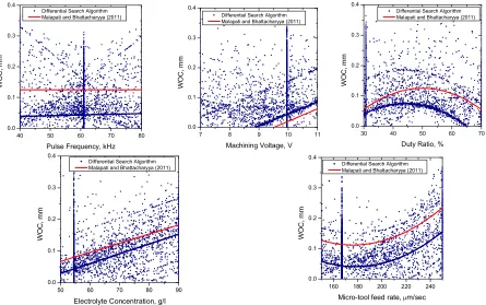
40 50 60 70 80 0.0 0.1 0.2 0.3 0.4

W

O

C

, mm

Pulse Frequency, kHz

7 8 9 10 11

0.0 0.1 0.2 0.3 0.4

WOC,

mm

Machining Voltage, V

30 40 50 60 70

0.0 0.1 0.2 0.3 0.4

WOC, mm

Duty Ratio, %

50 60 70 80 90

0.0 0.1 0.2 0.3 0.4

WOC,

mm

Electrolyte Concentration, g/l

160 180 200 220 240

0.0 0.1 0.2 0.3 0.4

WOC

,

mm

Micro-tool feed rate, m/sec

Fig. 3. Variations of WOC for different EMM process parameters

Multi-objective optimization

In multi-objective optimization, all the four responses are simultaneously optimized and for this, the following combined objective function is developed.

Minimize max 4 min 3 min 2 min 1 1 ) ( ) ( ) ( ) ( Z MRR Y w Linearity Y w LOC Y w WOC Y

w _WOC _LOC Linearity  _MRR

     

 , (7)

where YWOC, YLOC, YLinearityand YMRRare the RSM-based equations for WOC, LOC, Linearity and MRR

respectively as developed using the experimental data; w1, w2, w3 and w4 are the weight/priorities

assigned to WOC, LOC, Linearity and MRR respectively; and (WOC)min, (LOC)min, (Linearity)min and

(MRR)max are respectively the optimal values of the considered responses as obtained from the single

objective optimization results. The weights need to be assigned to the responses in such a way that they must add up to one. Sometimes, analytic hierarchy process may be helpful to determine the weight values to be allocated to the responses. In this case, equal weights, i.e. w1 = w2 = w3 = w4 =0.25, are

assigned to all the four responses. The same set of constraints as considered for single objective optimization is also used here for multi-objective optimization.

After solving the combined objective function of Eq. (7) using DSA, the multi-objective optimization results of Table 3 are obtained. It is observed that a combination of EMM process parameters given by pulse frequency = 80.0000 kHz, machining voltage = 8.3340V, duty ratio = 64.6364%, electrolyte concentration = 69.1625g/l and micro-tool feed rate = 181.4039μm/sec provides the simultaneously optimized values of the four responses as MRR = 4.8279 mg/min, WOC = 0.00006 mm, LOC = 0.0861

mm and linearity = 0.00053. The minimum objective function value (Z1) is achieved as -0.0341. After

(10)

where maximum MRR (3.1039 mg/min) and minimum values of accuracy (WOC of 0.0003 mm, LOC of 0.1676 mm and linearity of 0.0691) were achieved. It can be concluded that the optimal values of all the four responses as derived by DSA are far better than those achieved by Malapati and Bhattacharyya (2011) through their experiments.

Table 3

Multi-objective optimization results for Example 1

x1 x2 x3 x4 x5 WOC LOC Lin MRR

80.0000 8.3340 64.6364 69.1625 181.4039 6.03E-05 0.0861 5.33E-04 4.8279

4.2 Example 2

Munda and Bhattacharyya (2008) considered pulse on/off ratio, machining voltage, electrolyte concentration, voltage frequency and tool vibration frequency during EMM operation to investigate their effects on MRR and radial overcut (ROC) of the machined components. The experimentation plan was designed not only to obtain the optimal scheme for multi-variable experimentation, but also to perform studies for exploring the interactive and higher-order effects of various process parameters. A stainless steel wire of diameter 335μm was used as the micro tool for the experimentation and the workpiece specimens were 15×10×0.15 mm bare copper plates. A central composite half fraction second-order rotatable design with 32 experiments was adopted for studying the relationship between the process parameters and responses. The original values of EMM process parameters with their

corresponding levels are shown in Table 4. The developed RSM-based equations for MRR and ROC

are respectively given in Eqs. (5-6).

Table 4

EMM process parameters and their levels (Munda and Bhattacharyya, 2008)

−2 −1 0 +1 +2

Pulse on/off ratio (x1) 0.5 1.0 1.5 2.0 2.5

Machining voltage (x2) V 2.5 3.0 3.5 4.0 4.5

Electrolyte concentration (x3) g/l 10 15 20 25 30

Voltage frequency (x4) Hz 35 40 45 50 55

Tool vibration frequency (x5) Hz 100 150 200 250 300

YMRR= −1.78917 + 0.111858x1 + 1.36263x2 − 0.0864044x3+ 0.0231122x4 − 0.00139639x5 −

0.201666x12 − 0.0860582x22 − 0.000145752x32 − 0.000319532x42 + 3.893684×10-6x52 −

0.0704326x1x2 + 0.00838936x1x3 + 0.00275664x1x4 + 0.00178484x1x5 + 0.00870264x2x3 −

0.00700764x2x4− 0.00105004x2x5 + 0.00125437x3x4 + 0.0000247626x3x5 + 0.0000181174x4x5

(8)

YROC= −1.08149 + 1.21039x1 + 0.448639x2 − 0.0821333x3 + 0.0247783x4 − 0.00258589x5 +

0.0198541x12 + 0.0554876x22 + 0.00108447x32 + 0.000640329x42 + 2.817205×10-6x52 −

0.139966x1x2 − 0.00133867x1x3 − 0.0161759x1x4 − 5.41335×10-5x1x5 − 0:00307591x2x3 −

0.0163201x2x4 + 0:000831331x2x5 + 0.000786541x3x4 + 0.0000725981x3x5

− 6.94181×10-5x4x5

(9)

Single objective optimization

Now employing DSA, the RSM-based equations, as given in Eqns. (8)-(9) for the two responses, i.e. MRR and ROC, are separately optimized. In this case, MRR needs to be maximized while minimization of ROC is required. For optimizing the RSM-based equations for the two responses, the

constraints are set as 0.5 ≤ x1 ≤ 2.5, 2.5 ≤ x2 ≤ 4.5, 10 ≤ x3 ≤ 30, 35 ≤ x4 ≤ 55 and 100 ≤ x5 ≤ 300. The

(11)

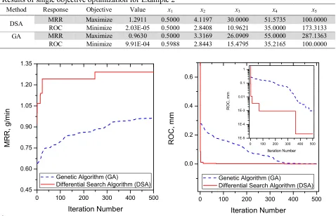
compares the optimal values of the responses as derived by DSA with those obtained by GA. It is again proved that DSA is superior to GA with respect to their optimization performance. Figure 4 shows the convergence of DSA and GA for the considered two responses. As Munda and Bhattacharyya (2008) did not perform any single objective optimization of the responses, so the optimal solutions as achieved applying DSA cannot be compared with those of the past researchers. The effects of various EMM process parameters on MRR and ROC are also observed through the developed scatter diagrams and the trends exactly match with those identified by Munda and Bhattacharyya (2008).

Table 5

Results of single objective optimization for Example 2

DSA MRR Maximize 1.2911 0.5000 4.1197 30.0000 51.5735 100.0000 ROC Minimize 2.03E-05 0.5000 2.8408 10.9621 35.0000 173.3133 GA MRR Maximize 0.9630 0.5000 3.3169 26.0909 55.0000 287.1363 ROC Minimize 9.91E-04 0.5988 2.8443 15.4795 35.2165 100.0000

0 100 200 300 400 500

0.45 0.60 0.75 0.90 1.05 1.20 1.35

MRR

, g

/m

in

Iteration Number

Genetic Algorithm (GA)

Differential Search Algorithm (DSA)

0 100 200 300 400 500

0.0 0.2 0.4 0.6

0 100 200 300 400 500

1E-5 1E-4 1E-3 0.01 0.1 1

ROC

, m

m

Iteration Number

R

OC, mm

Iteration Number

Genetic Algorithm (GA)

Differential Search Algorithm (DSA)

*

Multi-objective optimization

In order to simultaneously optimize both the responses, the following objective function of Eqn. (10) is developed:

Minimize 1 2

2

min max

,

( ) ( )

ROC MRR

w Y w Y

Z

ROC MRR

 

  (10)

where YROCand YMRRare the RSM-based equations for ROC and MRR respectively; w1 and w2 are the

weight/priorities assigned to ROC and MRR respectively; and (ROC)min and (MRR)max are respectively

the optimal values of the considered responses as obtained from the single objective optimization

results. Here, equal weights, i.e. w1 = w2 =0.50 are allocated to both the responses. From the results of

multi-objective optimization as obtained using DSA and shown in Table 6, it is observed that the maximum MRR value of 0.8354 g/min and minimum ROC value of 0.0097 mm are obtained at the

optimal combination of EMM process parameters of pulse on/off ratio = 0.5000, machining voltage =

4.0974V, electrolyte concentration = 30.0000g/l, voltage frequency = 47.0184 Hz and tool vibration

(12)

Munda and Bhattacharyya (2008) determined the maximum MRR value as 0.700 g/min and minimum ROC value as around 20μm at the optimal parametric combination of pulse on/off ratio = 1.0, machining voltage = 3 V, electrolyte concentration = 15g/l, voltage frequency = 42.118Hz and tool vibration frequency = 300 Hz. Thus, it can be claimed that while using DSA, the value of MRR is

increased from 0.700 g/min to 0.8354 g/min and the ROC value is drastically reduced from 20μm to 9μm.

Table 6

Results of multi-objective optimization for Example 2

x1 x2 x3 x4 x5 ROC MRR

0.5000 4.0974 30.0000 47.0184 300.0000 0.0097 0.8354

4.3 Example 3

After taking into consideration pulse on/off ratio, machining voltage, electrolyte concentration, voltage pulse frequency and tool vibration frequency as the five major EMM process parameters, Munda et al. (2007) studied their influences on micro-spark and stray-current affected zone (MSAZ) (in mm) of the machined surface. The value of MSAZ is quantified as the average difference between the hole radius to the distances between centre of the hole and different points along the curve that indicate the stray-current and micro-spark affected zone. Each of the EMM process parameters was set at five different levels, as given in Table 7. Based on a central composite half fraction second-order rotatable design plan and using the experimental data, the RSM-based regression equation, as given in Eqn. (11), was developed to study the interactive and higher-order effects of various EMM process parameters on MSAZ.

Table7

EMM process parameters and their levels (Munda et al., 2007)

−2 −1 0 +1 +2

Pulse on/off ratio (x1) 0.5 1.0 1.5 2.0 2.5

Machining voltage (x2) V 2.5 3.0 3.5 4.0 4.5

Electrolyte concentration (x3) g/l 10 15 20 25 30

Voltage frequency (x4) Hz 35 40 45 50 55

Tool vibration frequency (x5) Hz 100 150 200 250 300

YMSAZ = −0.418161 − 0.468499x1 − 0.0470149x2 + 0.122239x3 − 0.0330168x4 + 0.0121153x5 −

0.0685619x12 − 0.0267494x22 − 0.00218687x32 + 0.000838756x42 − 4.86869×10-6x52 + 0.0829706x1x2 +

0.01128426x1x3 + 0.00587294x1x4 − 0.000567606x1x5 + 0.0165958x2x3

− 0.000465437x2x4 − 0.00117664x2x5 − 0.00202633x3x4 − 7.65231×10 -5

x3x5 − 9.07856×10 -5

x4x5

(11)

The RSM-based equation depicting the interrelationship between various EMM process parameters and

MSAZ is now minimized with respect to the constraints set as 0.5 ≤ x1 ≤ 2.5, 2.5 ≤ x2 ≤ 4.5, 10 ≤ x3 ≤

30, 35 ≤ x4 ≤ 55 and 100 ≤ x5 ≤ 300. The results of single objective optimization obtained using DSA

and GA are exhibited in Table 8. Employing desirability function approach, Munda et al. (2007)

observed the optimal setting of various process parameters as pulse on/off ratio = 2.1618, machining

voltage = 2.8347 V, electrolyte concentration = 10 g/l, voltage frequency = 35 Hz and tool vibration

frequency = 100 Hz, and a minimum MSAZ value of 1×10-4 mm. From Table 8, it is found that the

minimum values of MSAZ are 4.1×10-7 mm and 1.23×10-4 mm respectively when the same

(13)

Table 8

Results of single objective optimization for Example 3

DSA MSAZ Minimize 4.1E-07 1.0750 4.5000 27.8550 45.8650 161.4100 GA MSAZ Minimize 1.23E-04 0.9758 3.8396 12.3990 43.4800 129.4400

0 100 200 300 400 500 0.0

0.2 0.4 0.6

0 100 200 300 400 500

1E-7 1E-6 1E-5 1E-4 1E-3 0.01 0.1 1

MSA

Z, mm

Iteration Number

MS

A

Z,

mm

Iteration Number

*

In this example, as there is only a single response, i.e. MSAZ, multi-objective optimization cannot be performed.

5. Conclusions

Forhaving enhanced MRR, better surface finish and surface integrity, it is always demanded that the

machining parameters of the EMM processes are set at their optimal values. In this paper, three examples leading to parametric optimization of EMM processes are considered and subsequently solved using DSA technique, which is an almost unexplored optimization tool for dealing with complex multi-modal mathematical functions. It is observed that in all the three cases, DSA provides better values of the considered responses (both for single and multi-objective optimization) when compared to those observed by the past researchers. When the optimization performance of DSA is compared with that of GA, the most popular population-based optimization method, it is again found that DSA outperforms GA in all the three examples. Not entirely depending upon the manufactures’ data or handbook data, the process engineers can now set the EMM processes at their optimal settings for having improved machining performance. As a future scope, the optimization performance of DSA can also be compared with that of other familiar evolutionary algorithms, like ACO, PSO, ABC, simulated annealing and biogeography-based optimization techniques. The applicability of DSA for parametric optimization of other non-traditional machining processes, like laser machining process, wire electric discharge machining process, plasma arc machining process, electro-chemical discharge machining process can also be experimented.

References

Bhattacharyya, B., Boloi, B., & Sridhar, P.S. (2001). Electrochemical micro-machining: new

possibilities for micro-manufacturing. Journal of Materials Processing Technology, 113(1-3),

301-305.

Bhattacharyya, B., Mitra, S., & Boro, A.K. (2002). Electrochemical machining: new possibilities for

(14)

Bhattacharyya, B., & Munda, J. (2003a). Experimental investigation on the influence of electrochemical

machining parameters on machining rate and accuracy in micromachining domain. International

Journal of Machine Tools & Manufacture, 43(13), 1301-1310.

Bhattacharyya, B., & Munda, J. (2003b). Experimental investigation into electrochemical

micromachining (EMM) process. Journal of Materials Processing Technology, 140(1-3), 287-291.

Bhattacharyya, B., Munda, J., & Malapati, M. (2004). Advancement in electrochemical

micro-machining. International Journal of Machine Tools & Manufacture, 44(15), 1577-1589.

Bhattacharyya, B., Malapati, M., & Munda, J. (2005). Experimental study on electrochemical

micromachining. Journal of Materials Processing Technology, 169(3), 485-492.

Bhattacharyya, B., Malapati, M., Munda, J., & Sarkar, A. (2007). Influence of tool vibration on

machining performance in electrochemical micro-machining of copper. International Journal of

Machine Tools & Manufacture, 47(2), 335-342.

Cao, G., Dai, Y., & Yao, L. (2012). Study on mechanism of electrochemical micro-machining of

titanium alloys. Applied Mechanics and Materials, 130-134, 2269-2272.

Civicioglu, P. (2012). Transforming geocentric Cartesian coordinates to geodetic coordinates by using

differential search algorithm. Computers & Geosciences, 46, 229-247.

Krebs, J.R. & Davies, N.B. (1997). Behavioural Ecology: An Evolutionary Approach, Cambridge, UK:

Blackwell Publishing.

Kurita, T., Chikamori, K., Kubota, S., & Hattori, M. (2006). A study of three-dimensional shape

machining with an ECμM system. International Journal of Machine Tools & Manufacture,

46(12-13), 1311-1318.

Li, Z., & Niu, Z. (2010). Process parameter optimization and experimental study of micro-holes in

electrochemical micromachining using pulse current. Advanced Materials Research, 135, 293-297.

Malapati, M., & Bhattacharyya, B. (2011). Investigation into electrochemical micromachining process

during micro-channel generation. Materials and Manufacturing Processes, 26(8), 1019-1027.

Malapati, M., Sarkar, A., & Bhattacharyya, B. (2011). Frequency pulse period and duty factor effects

on electrochemical micromachining (EMM). Advanced Materials Research, 264-265, 1334-1339.

Malapati, M., Sarkar, A., & Bhattacharyya, B. (2012). Micro-channel generation on copper-foil by

EMM process. International Journal of Machining and Machinability of Materials, 11(4), 385-404.

Mithu, M.A.H., Fantoni, G., & Ciampi, J. (2012). Fabrication of micro nozzles and micro pockets by

electrochemical micromachining. International Journal of Machining and Machinability of

Materials, 11(4), 353-370.

Munda, J., Malapati, M., & Bhattacharyya, B. (2007). Control of micro-spark and stray-current effect

during EMM process. Journal of Materials Processing Technology, 194(1-3), 151-158.

Munda, J., & Bhattacharyya, B. (2008). Investigation into electrochemical micromachining (EMM)

through response surface methodology based approach. International Journal of Advanced

Manufacturing Technology, 35(7-8), 821-832.

Munda, J., Malapati, M., & Bhattacharyya, B. (2010). Investigation into the influence of electrochemical micromachining (EMM) parameters on radial overcut through RSM-based

approach. International Journal of Manufacturing Technology and Management, 21(1/2), 54-66.

Rao, R.V., & Patel, V. (2012). An elitist teaching-learning-based optimization algorithm for solving

complex constrained optimization problems. International Journal of Industrial Engineering

Computations, 3(4), 535-560.

Samanta, S. & Chakraborty, S. (2011). Parametric optimization of some non-traditional machining

processes using artificial bee colony algorithm. Engineering Applications of Artificial Intelligence,

24, 946-957.

Thanigaivelan, R., & Arunachalam, R. (2013). Optimization of process parameters on machining rate

and overcut in electrochemical micromachining using grey relational analysis. Journal of Scientific

and Industrial Research, 72(1), 36-42.

Trianni, V., Tuci, E., Passino, K. & Marshall, J.R. (2011). Swarm Cognition: an interdisciplinary