University of New Orleans University of New Orleans
ScholarWorks@UNO
ScholarWorks@UNO
University of New Orleans Theses and
Dissertations Dissertations and Theses
Spring 5-23-2019
Modeling the Effect of a Compartment Fire on Spaces Adjacent to
Modeling the Effect of a Compartment Fire on Spaces Adjacent to
a Bulkhead With and Without Attachments
a Bulkhead With and Without Attachments
Carl E. Hendrickson II
University of New Orleans, [email protected]
Follow this and additional works at: https://scholarworks.uno.edu/td
Part of the Heat Transfer, Combustion Commons
Recommended Citation Recommended Citation
Hendrickson, Carl E. II, "Modeling the Effect of a Compartment Fire on Spaces Adjacent to a Bulkhead With and Without Attachments" (2019). University of New Orleans Theses and Dissertations. 2609. https://scholarworks.uno.edu/td/2609
This Thesis is protected by copyright and/or related rights. It has been brought to you by ScholarWorks@UNO with permission from the rights-holder(s). You are free to use this Thesis in any way that is permitted by the copyright and related rights legislation that applies to your use. For other uses you need to obtain permission from the rights-holder(s) directly, unless additional rights are indicated by a Creative Commons license in the record and/or on the work itself.
Modeling the Effect of a Compartment Fire on Spaces Adjacent to a Bulkhead, With and Without Attachments
A Thesis
Submitted to the Graduate Faculty of the University of New Orleans in partial fulfillment of the requirements for the degree of
Master of Science in Engineering Mechanical
by
Carl Hendrickson
B.S. United States Merchant Marine Academy, 2014
ii
Acknowledgement
I would like to convey my gratitude and respect for my thesis advisor, Dr. Martin Guillot.
He pushed me to properly research and produce a detailed and comprehensive report. I am thankful for
his constant guidance and feedback throughout this entire process.
I would also like to thank my wife, Maria, who always offered her unconditional support
throughout this program. She helped me to schedule my time efficiently and was always a source of
motivation.
Additionally, I would like to thank my parents for their endless support and love. They
taught me the importance of dedication and ambition, both of which were instrumental in putting together
this thesis.
Lastly, I would like to thank the University of New Orleans Master of Science in
Engineering program. The thorough graduate education I have received has made it possible to construct
iii
Table of Contents
List of Figures ... v
List of Tables ... x
Nomenclature ... xi
Abstract ... xiv
I. Introduction ... 1
II. Background ... 3
III. Literature Review ... 7
IV. Mathematical Modeling ... 21
A. Lumped Capacitance Model ... 22
1. Thermal Conductivity Model ... 27
2. Runge-Kutta Method ... 30
B. Lumped Capacitance Parallel Flow ... 32
C. CFD Model ... 37
1. Solver Theory ... 37
2. Fluent Convection ... 41
3. Physical Model ... 43
4. Governing Differential Equations and Boundary Conditions ... 45
5. Solution Procedure ... 48
6. Mesh Formulation ... 50
iv
A. Lumped Capacitance Model ... 52
B. CFD Model Baseline ... 55
1. Baseline Constant Thermal Conductivity ... 55
2. Baseline Temperature Dependent Thermal Conductivity ... 60
3. Mesh Independence Study ... 66
C. CFD Model with Attachment ... 81
1. 6.25 cm2 Fin ... 82
2. 25 cm2 Fin ... 90
3. 100 cm2 Fin ... 97
VI. Conclusion and Recommendations ... 104
References ... 105
v List of Figures
Figure II-1 Wire Hangers on Bulkhead ... 3
Figure III-1 E 119 Standard Fire Curve. Note. Reprinted from “A New Curve for Temperature-Time
Relationship in Compartment Fire”, by Blagojevic, M., 2011, Thermal Science, 15, p. 342. ... 7
Figure III-2 Idealized Fire Curve. Note. Reprinted from SFPE Handbook of Fire Protection Engineering
(4-201), by T. T. Lie, 2002, Bethesda, Maryland: National Fire Protection Association. ... 9
Figure III-3 Set up for TPS Method. Note. Reprinted from “Measurement of thermal properties at
elevated temperatures”, by Jansson, R., 2004, Swedish National Testing and Research Institute, p. 15. .. 10
Figure III-4 Thermal Conductivity of Steel and Temperature. Reprinted from Fire Design of Steel
Structures (321), by J. Franssen and P.V. Real, 2012, European Convention for Constructional Steelwork.
... 11
Figure III-5 80 x 80 Inflation on Walls of Square Cavity. Note. Reprinted from “Simulation of
Steady-State Natural Convection Using CFD”, by Zitzmann, T. et al., 2005, Building Simulation, p. 1451. ... 13
Figure III-6 3-D Enclosure Geometry and Boundary Conditions. Note. Reprinted from “A numerical
study of 3D natural convection in a cube: effects of the horizontal thermal boundary conditions”, by
Fusegi, T. et al., 1991, Fluid Dynamics Research, 8, p. 222. ... 14
Figure III-7 1-D Model for Heat Conduction. Note. Reprinted from “Temperature Analysis of
Heavily-Insulated Steel Structures Exposed to Fires”, by Wickstrom, U., 1985, Fire Safety Journal, 9, p. 281. .... 15
Figure III-8 1-D Condensed Heat Transfer Model. Note. Reprinted from “Modified One Zone Model for
... 16
Figure III-9 FEM Model. Note. Reprinted from “Modified One Zone Model for Fire Resistance Design of
Steel Structures”, by Zhang, C., 2012, Advanced Steel Construction, 9, p. 290. ... 16
Figure III-10 Small Scale Horizontal Exposure Furnace/Underwriter’s Laboratories 1 m Furnace. Note.
Reprinted from “Fire Resistance Testing of Bulkhead and Deck Penetrations”, by Beene, D. et al., Year,
vi
Figure III-11 Test Piece for Fire Test Note. Reprinted from “Fire Resistance Testing of Bulkhead and
Deck Penetrations”, by Beene, D. et al., Year, Marine Safety Laboratories, p. C-15... 19
Figure IV-1 Lumped Capacitance Model ... 22
Figure IV-2 Lumped Capacitance Heat Flux Insulation ... 23
Figure IV-3 Lumped Capacitance Heat Flux Steel ... 23
Figure IV-4 Lumped Capacitance Heat Flux Air ... 23
Figure IV-5 Thermal Conductivity vs. Temperature of Insulation. Adapted from “Measurement of thermal properties at elevated temperatures”, by Jansson, R., 2004, Swedish National Testing and Research Institute, p. 89. ... 28
Figure IV-6 Thermal Conductivity vs. Temperature of Steel. Adapted from Fire Design of Steel Structures (321), by J. Franssen and P.V. Real, 2012, European Convention for Constructional Steelwork. ... 29
Figure IV-7 Lumped Capacitance Parallel Flow Model ... 32
Figure IV-8 Lumped Capacitance Heat Flux Attachment ... 33
Figure IV-9 Lumped Capacitance Heat Flux Insulation ... 34
Figure IV-10 Lumped Capacitance Heat Flux Steel ... 34
Figure IV-11 Lumped Capacitance Heat Flux Air ... 35
Figure IV-12 Control Volume for Discretization of Scalar Transport Equation. Reprinted from “ANSYS Fluent Theory Guide”, p. 18-9. ... 40
Figure IV-13 Fluid and Solid Region, CFD Model ... 43
Figure IV-14 Fluid Region, CFD Model ... 44
Figure IV-15 Solid Region, CFD Model ... 44
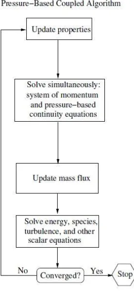
Figure IV-16 Pressure-Based Solution Method. Reprinted from “ANSYS Fluent Theory Guide”, p. 18-4. ... 48
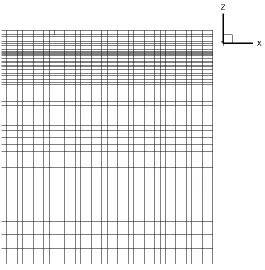
Figure IV-17 Mesh Bias ... 50
vii
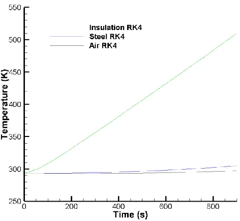
Figure V-1 Lumped Capacitance Results ... 52
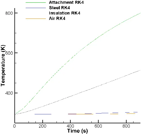
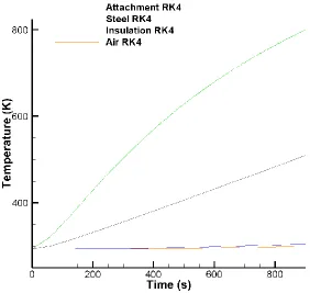
Figure V-2 Lumped Capacitance Parallel Flow, 6.25 cm2 Attachment Results ... 53
Figure V-3 Lumped Capacitance Parallel Flow, 25 cm2 Attachment Results ... 53
Figure V-4 Lumped Capacitance Parallel Flow, 100 cm2 Attachment Results ... 54
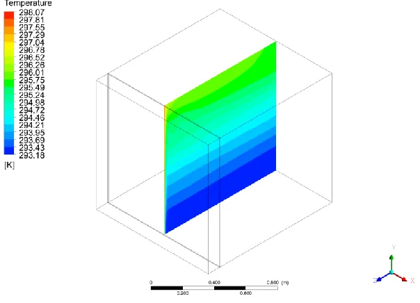
Figure V-5 Baseline Model Side View Temperature Contour, Constant Thermal Conductivity ... 55
Figure V-6 Baseline Model Isometric View Temperature Contour, Constant Thermal Conductivity ... 55
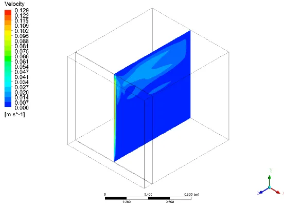
Figure V-7 Baseline Model Side View Velocity Contour, Constant Thermal Conductivity ... 56
Figure V-8 Baseline Model Isometric View Velocity Contour, Constant Thermal Conductivity ... 56
Figure V-9 Baseline Model Side View Temperature Contour Air, Constant Thermal Conductivity ... 57
Figure V-10 Baseline Model Isometric View Temperature Contour Air, Constant Thermal Conductivity ... 57
Figure V-11 CFD vs Lumped Capacitance Results, Constant Thermal Conductivity ... 58
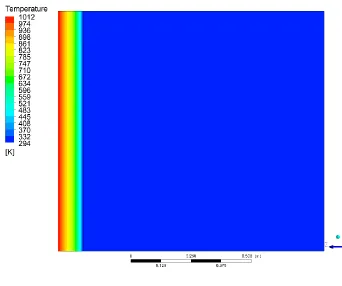
Figure V-12 Baseline Model Side View Temperature Contour ... 60
Figure V-13 Baseline Model Isometric View Temperature Contour ... 61
Figure V-14 Baseline Model Side View Velocity Contour ... 61
Figure V-15 Baseline Model Isometric View Velocity Contour ... 62
Figure V-16 Baseline Model Side View Temperature Contour Air ... 62
Figure V-17 Baseline Model Isometric View Temperature Contour Air ... 63
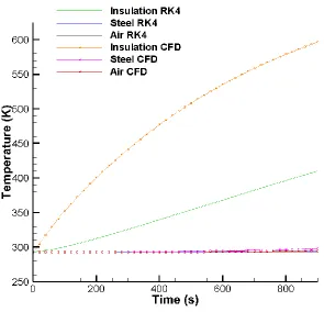
Figure V-18 Baseline CFD vs Lumped Capacitance Results ... 64
Figure V-19 Baseline Coarse Mesh Side View Temperature Contour ... 67
Figure V-20 Baseline Coarse Mesh Isometric View Temperature Contour ... 67
Figure V-21 Baseline Coarse Mesh Side View Velocity Contour ... 68
Figure V-22 Baseline Coarse Mesh Isometric View Velocity Contour ... 68
Figure V-23 Baseline Coarse Mesh Side View Temperature Contour Air ... 69
Figure V-24 Baseline Coarse Mesh Isometric View Temperature Contour Air ... 69
viii
Figure V-26 Baseline Fine Mesh Isometric View Temperature Contour ... 70
Figure V-27 Baseline Fine Mesh Side View Velocity Contour ... 71
Figure V-28 Baseline Fine Mesh Isometric View Velocity Vector ... 71
Figure V-29 Baseline Fine Mesh Side View Temperature Contour Air ... 72
Figure V-30 Baseline Fine Mesh Isometric View Temperature Contour Air ... 72
Figure V-31 Baseline 0.25 Second Time-step Side View Temperature Contour ... 73
Figure V-32 Baseline 0.25 Second Time-step Isometric View Temperature Contour ... 74
Figure V-33 Baseline 0.25 Second Time-step Side View Velocity Contour ... 74
Figure V-34 Baseline 0.25 Second Time-step Isometric View Velocity Contour ... 74
Figure V-35 Baseline 0.25 Second Time-step Side View Temperature Contour Air ... 75
Figure V-36 Baseline 0.25 Second Time-step Isometric View Temperature Contour Air ... 75
Figure V-37 Baseline 1 Second Time-step Side View Temperature Contour ... 76
Figure V-38 Baseline 1 Second Time-step Isometric View Temperature Contour ... 76
Figure V-39 Baseline 1 Second Time-step Side View Velocity Contour ... 77
Figure V-40 Baseline 1 Second Time-step Isometric View Velocity Contour ... 77
Figure V-41 Baseline 1 Second Time-step Side View Temperature Contour Air ... 78
Figure V-42 Baseline 1 Second Time-step Isometric View Temperature Contour Air ... 78
Figure V-43 Comparison of Temperature along CL for Different Meshes ... 79
Figure V-44 Comparison of Temperature along CL for Different Time Steps ... 79
Figure V-45 6.25 cm2 Attachment Side View Temperature Contour ... 82
Figure V-46 6.25 cm2 Attachment Isometric View Temperature Contour ... 83
Figure V-47 6.25 cm2 Attachment Side View Velocity Contour ... 83
Figure V-48 6.25 cm2 Attachment Isometric View Velocity Contour ... 84
Figure V-49 6.25 cm2 Attachment Side View Temperature Contour Air ... 85
Figure V-50 6.25 cm2 Attachment Isometric View Temperature Contour Air ... 85
ix
Figure V-52 6.25 cm2 Attachment Steel Bulkhead Air-side View Temperature Contour ... 86
Figure V-53 6.25 cm2 Attachment Steel Bulkhead Isometric View Temperature Contour ... 87
Figure V-54 6.25 cm2 Attachment Temperature along Centerline ... 87
Figure V-55 6.25 cm2 Attachment CFD Results vs Lumped Capacitance Parallel Flow ... 88
Figure V-56 25 cm2 Attachment Side View Temperature Contour ... 90
Figure V-57 25 cm2 Attachment Isometric View Temperature Contour ... 90
Figure V-58 25 cm2 Attachment Side View Velocity Contour ... 91
Figure V-59 25 cm2 Attachment Isometric View Velocity Contour ... 91
Figure V-60 25 cm2 Attachment Side View Temperature Contour Air ... 92
Figure V-61 25 cm2 Attachment Isometric View Temperature Contour Air ... 93
Figure V-62 25 cm2 Attachment Zoomed View Temperature Contour Air ... 93
Figure V-63 25 cm2 Attachment Steel Bulkhead Temperature Contour ... 94
Figure V-64 25 cm2 Attachment Steel Bulkhead Isometric View Temperature Contour ... 94
Figure V-65 5 cm2 Attachment Temperature along Centerline ... 95
Figure V-66 25 cm2 Attachment CFD Results vs Lumped Capacitance Parallel Flow ... 95
Figure V-67 100 cm2 Attachment Side View Temperature Contour ... 97
Figure V-68 100 cm2 Attachment Isometric View Temperature Contour ... 97
Figure V-69 100 cm2 Attachment Side View Velocity Contour ... 98
Figure V-70 100 cm2 Attachment Isometric View Velocity Contour ... 98
Figure V-71 100 cm2 Attachment Side View Temperature Contour Air ... 99
Figure V-72 100 cm2 Attachment Isometric View Temperature Contour Air ... 100
Figure V-73 100 cm2 Attachment Zoomed View Temperature Contour Air ... 100
Figure V-74 100 cm2 Attachment Steel Bulkhead Temperature Contour ... 101
Figure V-75 100 cm2 Attachment Steel Bulkhead Isometric View Temperature Contour ... 101
Figure V-76 100 cm2 Attachment Temperature along Centerline ... 102
x List of Tables
Table IV-1 Temperature vs. Thermal Conductivity of Insulation. Adapted from “Measurement of thermal
properties at elevated temperatures”, by Jansson, R., 2004, Swedish National Testing and Research
Institute, p. 86. ... 27
Table IV-2 CFD Solver Settings ... 49
Table V-1 Temperatures of Elements after 15 minutes ... 52
Table V-2 Mesh Independence Study ... 66
Table V-3 Mesh Independence Study Temperature Averages ... 66
xi Nomenclature
(
x y z
, ,
)
Cartesian Coordinates(
u v w
, ,
)
Velocity ComponentsH Height
( )
m
L Length
( )
m
g Gravitational Acceleration
(
m s
/
2)
T Temperature ( )K
p Pressure (Pa)
h
Convection Coefficient(
W m K/ 2)
V
Volume( )
m3p
c Specific Heat ( /J kgK)
m
mass (kg)1
i
T
Surface temperature of fire side surface of insulation (function of time) ( )K, ,
s i a
T T T Temperature of steel, insulation, and air (function of time) ( )K
Thermal Conductivity (W mK/ )
Average Thermal Conductivity (W mK/ )xii w
M
Molecular Weight of Gas"
q Heat Flux, Heat Transfer per Unit Area (W m/ 2)
Pr Prandtl number
Gr Grashof number
Bi Local Convective Heat Transfer Parameter
Ra Rayleigh number
Nu Nusselt number
Re Reynolds number
Lumped Capacitance
0
q
Heat Transfer from Fire to Insulation( )
W
1
q
Heat Transfer Insulation to Steel( )
W
2
q
Heat Transfer Steel to Air( )
W
Lumped Capacitance Parallel Flow
0
q
Heat Transfer from Fire to Attachment( )
W
1
q
Heat Transfer from Attachment to Air( )
W
2
q
Heat Transfer from Fire to Insulation( )
W
3
q
Heat Transfer from Insulation to Steel( )
W
4
xiii
1
s
Attachment2
s
SteelT
L Length of Attachment
Greek Symbols
Viscosity (kg ms/ )
Kinematic Viscosity(
m
2/ )
s
Thermal Diffusivity(
m
2/ )
s
Thermal Expansion Coefficient (1 /K)
Density(
kg m
/
3)
Subscript
i insulation
s
steela
airf fire
xiv Abstract
Structural fire protection is an integral component of shipboard fire safety. There are national and
international regulations that delineate requirements for the insulation placed throughout ships. The
attachments that penetrate the insulation for hanging wires and pipes can disrupt the integrity of the
division, and cause a failure to adhere to the regulations. This problem will be analyzed by using a
simplified lumped capacitance model and ANSYS FLUENT CFD. A standard time-temperature fire
curve is applied to the fire side of the enclosure. The thermal conductivity of the insulation and steel are
made to be temperature dependent. The density of the air of the non-fire side is then approximated using
the Boussinesq approximation for lower temperature differences and the incompressible ideal gas law for
higher temperature differences. Different attachments of varying surface areas and volumes are exposed
to the standard time-temperature fire curve and their heat transfer capabilities are analyzed.
Keywords: fire safety, insulation, fire curve, ship safety, CFD, lumped capacitance, Boussinesq
1 I. Introduction
Safety is vital in the proper functioning of vessels and adequate protection of both people and
materials aboard ships. Among the various threats to shipboard safety, fires are some of the most
devastating disasters that can lead to loss of both life and property. As a result, this has led to the
implementation of broad regulations for ships to maintain a minimum standard of safety in regard to fire
protection.
The regulations regarding fire control boundaries can be found in SOLAS (Safety of Life at Sea)
Chapter II-2 and CFR (Code of Federal Regulations) 46. CFR considers the provisions provided by
SOLAS to be equivalent to their own federal regulations. SOLAS states the requirements for the
constraints of bulkheads and decks, but also references the FTP (Fire Testing Procedure) Code for
methods regarding testing the materials.
The purpose of SOLAS in regard to its requirement for fire safety is to “prevent the occurrence of
fire and explosion; reduce the risk to life caused by fire; reduce the risk of damage caused by fire to the
ship, its cargo and the environment; contain, control and suppress fire and explosion in the compartment
of origin, and provide adequate and readily accessible means of escape for passengers and crew” (SOLAS
Consolidated Edition, 2014).
In order to properly implement these regulations, each vessel needs to have emergency
arrangements in place in order to combat fires. Additionally, the crew must be trained in firefighting and
have ample, competent fireteams to effectively combat a potential fire. Lastly, there needs to be installed
passive fire protection and fire suppression systems (SOLAS Consolidated Edition, 2014).
The passive fire protection is accomplished onboard a ship through insulation. The bulkheads and
decks of ships are made to be resistant to fire. However, the multiple penetrations for hanging wires,
2
properly, there can be a disruption in their integrity and a failure of the ship’s fire suppression
capabilities, potentially inducing a catastrophic loss of property and life (Beene et al., 1988).
This thesis studies attachments. Attachments and penetrations are very similar. A penetration
goes not only through the insulation, but also through the steel bulkhead or deck. An attachment will only
go through the insulation and then be attached to the steel itself. Attachments raise the same concerns for
the temperature requirements on the non-fire side, but are less likely to cause the passage of smoke and
flame to the non-fire side because they do not cut into the bulkhead. Although SOLAS does not speak
specifically to attachments, it is assumed that the regulations for penetrations are equivalent.
The United States Coast Guard (USCG) has reported that some shipbuilders have raised concerns
regarding the necessity of insulating attachments (C. Briggs, personal communication, April 30, 2018).
Shipbuilders claim that attachments are too insignificant to cause a failure of the regulations and therefore
do not pose a danger to ships when there is a fire onboard. These shipbuilders state that insulating the
attachments is an unnecessary costly expenditure in terms of money, resources, and time. They maintain
that the fire divisions can meet the criteria stated by the regulations without insulating these attachments.
However, the regulations claim that attachments are significant and crucial to the fire protection system
(SOLAS Consolidated Edition, 2014). This study explores the implications of attachments without
3 II. Background
Ship fire regulations are complex and encompass many different components. Each physical
division aboard a ship, including bulkheads and decks, is split into different classes that have separate
requirements in regard to shipboard fire safety.
Figure II-1 Wire Hangers on Bulkhead
Figure II-1 illustrates how various attachments could harm the integrity of the fire resistance in
any given bulkhead. The USCG specifically requires coat-back, a spray-on insulation, to be applied to the
attachments if they cannot meet the criteria for their boundary alone.
Each bulkhead and deck on a ship is then classified as A-60, A-30, A-15, A-0, B-15, B-0, C, or
C'. Depending on the location, a bulkhead will need to provide different criteria for its resistance to a fire.
The “A” class division has the most stringent of criteria. “‘A’ class divisions are those divisions formed
by bulkheads and decks which comply with the following criteria: they are constructed of steel or other
equivalent material; they are suitably stiffened; they are insulated with approved non-combustible
materials such that the average temperature of the unexposed side will not rise more than 140o C above
the original temperature, nor will the temperature, at any one point, including any joint, rise more than
4
has to maintain these standards for a total of 60 minutes. The “A” class division is then decreased in the
time constraints for A-30, A-15, and A-0. This means that these divisions must meet the criteria for A-60
as previously stated, but for 30 minutes, 15 minutes, and 0 minutes, respectively (SOLAS Consolidated
Edition, 2014).
SOLAS then goes on to describe how penetrations through fire boundaries should be treated.
“Where a[n] “A” class division is penetrated, the penetration shall be tested in accordance with the FTP
Code” (SOLAS Consolidated Edition, 2014). The United States accepts the testing procedures laid out in
ASTM E-119 as an equivalent to the FTP Code (NVIC 9-97, 2010).
The next lower standard for the fire resistance of a bulkhead and deck is the “B” class division.
Within this class, materials must be non-combustible like in the “A” class, however the difference
between the two is with the temperature threshold. “B” class materials “have an insulation value such that
the average temperature of the unexposed side will not rise more than 140o C above the original
temperature, nor will the temperature at any one point, including any joint, rise more than 225o C above
the original temperature” (SOLAS Consolidated Edition, 2014, p. 126). B-15 boundaries must conform to
these regulations for 15 minutes, and B-0 for 0 minutes. In terms of penetrations, “arrangements shall be
made to ensure that the fire resistance [within the ‘B’ division] is not impaired” (SOLAS Consolidated
Edition, 2014, p.168).
The United States Coast Guard provides directives in order to explain the complicated regulations
for the shipping industry. In regard to shipboard fire protection, the Coast Guard’s provided directive is
NVIC 9-97. NVIC 9-97 explains the procedure for testing structural fire protection. The regulation is as
follows:
“The required type approval tests for A-60 structural insulations are described in
46 CFR 164.007. All materials submitted for approval in this category must first pass the
required test for noncombustible materials under 46 CFR 164.009. 46 CFR 164.007 is a
5
by 60 in) specimen subjected to a one-hour fire exposure. In the test, the insulation is
applied to a 5 mm (3/16 inch) steel plate that is mounted in the test furnace with the
insulation exposed to the fire. The furnace is then controlled at the ASTM E-119 standard
time temperature curve for a one-hour period. The acceptance criteria require that the
insulation must prevent the passage of flame and the emission of appreciable volumes of
smoke and toxic gases from the unexposed surface during the 60 minute test period, and
must also prevent the temperature on the unexposed side of the bulkhead from exceeding
an average temperature rise of 139o C (250º F) above ambient, and a maximum
temperature rise of 180o C (325º F) above ambient at any one thermocouple.” (NVIC
9-97, 2010, p. 20)
Most of the modeling included in this thesis will be based off of the measurements mentioned in
the above regulation.
United States regulations for the ASTM Standard E-119 test methods are equivalent to the IMO
International Maritime Organization (IMO) Fire Testing Procedures (FTP). For the E-119 method, the test
fire specimen panel, which includes physical divisions like bulkheads and decks, is set on one face of a
test furnace. The furnace is then fired, and the rate of temperature produced is controlled by a
standard-time temperature curve (NVIC 9-97, 2010).
( )
345log (8
101) 20
f
T
t
=
t
+ +
(0.1)The E-119 test then measures the fire resistance of the specimen until failure. Failure occurs when
there is passage of smoke or flame or there is excessive heat transmission through the specimen.
There are also standards specifically testing the fire resistance of penetrations. These standards
are ASTM E-814 and UL 1479; both of these tests incorporate the standard time-temperature curve from
6
In order to provide a model to research this topic, a plethora of heat transfer aspects need to be
combined. These topics include time-dependent fire curves, temperature-dependent thermal material
properties at elevated temperatures, and buoyancy-driven convective flow. For the proposed model, the
fire curve is driving a temperature on the surface of the insulation, and provides a boundary condition for
the models. The temperature of the insulation, penetration, and steel will then increase, and, as the
temperature is elevated, their thermal conductivity changes. This in turn heats the air for the adjacent
space to the fire. The buoyancy-driven convection displaces the heat throughout the room, and a viscous
and thermal boundary layer is formed at the steel. This study combines these factors to provide a model
and determine whether or not a non-insulated penetration causes a failure of the regulations.
The purpose of this study is to determine if insulating attachments that penetrate fire divisions is
necessary. In order to prove the necessity of the insulation, a model is created where a non-insulated
attachment is present. This model is then evaluated to determine if it conforms to the regulations. This
study evaluates varying surface areas exposed to the standard time temperature curve for a total of 15
minutes. If insulating them is significant to the fire division’s integrity, then this study will reinforce the
regulations. If not, then further studies and experimentation will need to be conducted to determine the
7 III. Literature Review
Shipboard fires can be highly devastating and can easily end in the loss of property and life. A
ship’s passive fire protection and active fire protection are both highly complex systems that are subject to
national and international regulations. In order to make a model compatible for a shipboard fire, the first
item that needs to be simulated is the behavior of the fire. According to the United States Coast Guard’s
NVIC 9-97, when PFP is tested, the temperature of the fire should be controlled by ASTM’s 119.
E-119 proposes a standard fire curve of the form:
( )
345log10(
8 1)
20f
T t = t+ + (1.1)
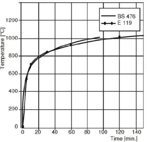
Figure III-1 E 119 Standard Fire Curve. Note. Reprinted from “A New Curve for Temperature-Time
Relationship in Compartment Fire”, by Blagojevic, M., 2011, Thermal Science, 15, p. 342.
Figure III-1 shows the standard fire curve where the temperature, T is the average furnace
temperature in degrees Celsius and
t
is time in minutes. According to NVIC 9-97 and the Fire Test8
structural insulations, bulkhead panels, doors, windows, fire dampers, and penetration seals determines if
they qualify as “A” class or “B” class divisions. A specimen of the material is mounted in a full-scale
laboratory furnace with gas burners that are controlled to expose the test specimen to flames and heat that
follow a standard time-temperature curve (NVIC 9-97, 2010).
Studies have been conducted to challenge the accuracy of this fire curve. Blagojevic and Pesic
(2011) claim that the standard fire curve does not include all the phases of a fire. According to their
research, “a proper fire curve includes three distinct phases: a growth phase, which is the development
phase from ignition to flashover, a steady-burning (fully developed) phase, and a decay phase”
(Blagojevic and Pesic, 2011). The growth phase is not perfectly modeled within the standard fire curve. In
addition, the decay phase is not represented adequately (Blagojevic and Pesic, 2011).
The SFPE Handbook of Fire Protection (2008) depicts an idealized fire curve that encompasses
these three phases. The Handbook also explains the phenomena that occurs during the different phases.
The first phase of the fire is the growth period. During this phase, heat begins to accumulate in the
enclosure. This accumulation can cause other materials in the room to ignite as well. This phenomenon is
situational and wholly depends on the materials immediately available; in terms of ships, these materials
generally include steel, paint, and fuel oil, and can influence the temperature and growth of the fire.
During the growth phase, there is dramatic rise in the gas temperatures which will result in a flashover.
Flashover can be defined as, “A transition in the development of a compartment fire when surfaces
exposed to thermal radiation from fire gases in excess of 1100°F reach ignition temperature more or less
simultaneously. This causes the fire to spread rapidly throughout the space, resulting in fire involvement
of the entire compartment or enclosed space” (Firefighting Procedures, 2010). Once flashover occurs,
then the steady-burning or fully developed phase begins. With this idealized curve in mind, the
temperature during the growth phase is relatively low and it can be assumed that the influence on the fire
resistance is negligible. Therefore, the actual risk begins during the steady-burning phase. During the
steady-burning phase, temperatures in excess of 1000o C can be attained. This excessive and dramatic
9
attachments. It is important to note that this risk of the excessive increase in temperature can still occur
during the decay phase (SFPE Handbook of Fire Protection, 2008, p. 4-201).
Figure III-2 Idealized Fire Curve. Note. Reprinted from SFPE Handbook of Fire Protection Engineering
(4-201), by T. T. Lie, 2002, Bethesda, Maryland: National Fire Protection Association.
Figure III-2 shows the idealized fire curve and has proper representation of the three periods of a
fire. The standard fire curve is more robust and experiences on-average higher temperatures than a curve
representing the three phases of a fire. The standard fire curve is also still stated as the acceptable fire
curve in the Coast Guard’s NVIC 9-97 and the International Maritime Organization’s (IMO) FTP Code.
The next important aspect of modeling a shipboard fire is to evaluate the thermal properties of
insulation and steel. There are various materials used for insulation, but a commonly used one for ships is
mineral wool. Budaiwi and Abdou (2005) concluded that the thermal conductivity of mineral wool
increases with an increase in temperature. The thermal conductivity is also proportional to the density of
the mineral wool. To determine this, Jansson (2004) used two different types of sensors: Kapton and
Mica. In this study, there was a discrepancy between the measurements taken between the two sensors;
10
sensor took measurements at higher temperatures for the thermal properties. Therefore, these
measurements were used for this thesis. This study uses the TPS (Transient Plane Source) method, which
incorporates the Mica sensor, in order to determine the thermal properties of mineral wool. The thermal
conductivity, diffusivity, and the volumetric specific heat were found at room temperature and at elevated
temperatures (Jansson, 2004).
The TPS method is performed by placing a flat round hot disc sensor between two pieces of a
material, as shown in Figure III-3.
Figure III-3 Set up for TPS Method. Note. Reprinted from “Measurement of thermal properties at
elevated temperatures”, by Jansson, R., 2004, Swedish National Testing and Research Institute, p. 15.
The sensor is constructed of a thin nickel foil spiral, which is 10 µm thick and is placed in
between two sheets of electrical insulation material. The hot disc sensor then acts as a constant effect
generator and a resistance thermometer simultaneously. The beginning of the measurement starts with a
stepwise power pulse being applied to the sensor. Then, when a constant electrical effect is applied, the
temperature rises in the sensor and heat flows to the tested material. The time-dependent resistance rise is
recorded and converted with a temperature coefficient of resistivity for nickel to a temperature response
11
The temperature rise in the sensor is related to the thermal properties of the tested material. In the
case of the material having good insulation properties, low conductivity and diffusivity, the temperature
of the sensor will rapidly rise with heat being applied. When the material has good conducting properties,
the heat will be transported faster inside the material, resulting in a lower rise in temperature for the
sensor. Jansson’s research aptly shows how temperature affects the thermal conductivity of mineral wool.
The findings from his work are important for modeling insulation at elevated temperatures (Jansson,
2004).
After the temperature of the fire affects the thermal properties of the insulation, the fire curve
temperature will then affect the steel of the bulkhead. The thermal properties of the steel need to be
examined. Figure III-4 shows the thermal conductivity of steel and the effect of increasing temperature.
Franssen and Real (2012) evaluate the thermal properties of carbon steel and propose algebraic relations
for the time-temperature dependence.
Figure III-4 Thermal Conductivity of Steel and Temperature. Reprinted from Fire Design of Steel
12 When
T
s
1073.5
K
then;54 0.033(Ts 273.15)
= − − (1.2)When
T
i
873.15
K
then;0.0009Ti 0.425835
= − (1.3)The topics of natural convection in 3-D enclosures and the thermal and viscous boundary layers
produced on vertical walls have been studied extensively by many researchers: Makinde and Olanrewaju
(2010), Baskak et al. (2006), and Zitzmann et al. (2005). Natural convection is caused by buoyancy forces
in an enclosure. Buoyancy occurs when heat is added to a fluid causing a change in fluid density. A flow
will then be induced by gravity acting upon the density variations. These buoyancy-driven flows are
called natural-convection or mixed-convection. Convection Heat Transfer by Arpaci and Larsen (1984)
provides a concise explanation of buoyancy driven flows. They state that the most frequently encountered
buoyancy is due to gravity and is seen in the heating and cooling of spaces. “The other type of buoyancy
driven flow is due to centrifugal forces, which is commonly observed in the cooling of turbine blades and
inertial forces, which has an impact on the cryogenic liquids in accelerating rockets” (Convection Heat
Transfer, 1984).
Many researchers have studied thermal boundary layers and convection occurring on flat vertical
plates and in square enclosures. According to Makinde and Olanrewaju (2010), when there is an increase
in the Prandtl number and the Grashof numbers, there is a decrease in the thermal boundary layer
thickness. Below are the equations for the Prandtl and Grashof numbers.
Pr
13
=
(1.5)(
)
2
f
xg
T
T
Gr
U
−
=
(1.6)An increase in temperature at the wall will therefore cause the density of air to decrease. This
decrease in density causes thermal boundary layer thickness to decrease as well.
Natural convection in a square cavity has also been investigated thoroughly. Baskak et al. (2006)
demonstrates the formation of thermal boundary layers with both uniform and non-uniform heating at the
wall. They found that the thermal boundary layer formed from non-uniform heating is less than that
developed from uniform heating. Zitzmann et al. (2005) concluded in their study of natural convection
that, at the walls of an enclosure, a significant inflation factor or bias is required, like in Figure III-5, in
order to obtain convergence.
Figure III-5 80 x 80 Inflation on Walls of Square Cavity. Note. Reprinted from “Simulation of
Steady-State Natural Convection Using CFD”, by Zitzmann, T. et al., 2005, Building Simulation, p. 1451.
Fusegi et al. (1991) proposed natural convection in a 3-D enclosure. In this study, the boundary
conditions at the walls were varied. The boundary conditions of the walls were varied by either being
14
this air-filled 3-D enclosure were computed at Rayleigh numbers of 105 and 106. The authors discussed
how, through computations, it is relatively easy to specify clearly defined boundary conditions; however,
it is much more difficult to achieve the same results through well-controlled experiments. For example, in
an actual experiment, a perfect insulator at a wall cannot be realized. Also, heat transfer through adiabatic
surfaces is always present, which causes direct comparisons between computations and experimental
results difficult. Therefore, in order to compare the two results, they are limited to the difference between
idealized computational conditions and real experimental situations. An example for the boundary
conditions of a 3-D enclosure with the varying boundary conditions can be shown in Figure III-6.
Figure III-6 3-D Enclosure Geometry and Boundary Conditions. Note. Reprinted from “A numerical
study of 3D natural convection in a cube: effects of the horizontal thermal boundary conditions”, by
Fusegi, T. et al., 1991, Fluid Dynamics Research, 8, p. 222.
Fusegi et al. (1991) concluded that the adiabatic and perfectly conducting boundary conditions on
the horizontal walls greatly influence the flow inside the enclosure. When heat transfer was allowed at the
15
The final aspect to analyze is the combination of the last three topics of discussion: fire modeling
for enclosures. Wickstrom et al. (2007) introduces an adiabatic surface temperature as a means to transfer
data from fire models to thermal/structural models. The authors state that the adiabatic surface
temperature can be obtained as an output from a fire model, and that it can be measured in real fire tests
or experiments by the use of a plate thermometer. Therefore, the adiabatic surface temperature would be
measured by an ideal plate thermometer. The plate thermometer is used in fire resistance testing (E119
and ISO834) to control the furnace temperature. The temperature measured by the plate thermometer is
required in the calculation of the exposed structural element.
Wickstrom (1985) analyzed the temperature of heavily insulated steel structures that were
exposed to fire. He applied the ISO 834 Fire Curve to the insulation surface and crafted a 1-D model,
Figure III-7, for conductive heat transfer.
Figure III-7 1-D Model for Heat Conduction. Note. Reprinted from “Temperature Analysis of
Heavily-Insulated Steel Structures Exposed to Fires”, by Wickstrom, U., 1985, Fire Safety Journal, 9, p. 281.
His research concluded that the material properties at elevated temperatures were a necessary
aspect for finding the temperature of the insulation and steel.
Zhang and Li (2012) presented a 1-D model with the addition of radiation and convection, as seen
16
Figure III-8 1-D Condensed Heat Transfer Model. Note. Reprinted from “Modified One Zone Model for
Fire Resistance Design of Steel Structures”, by Zhang, C., 2012, Advanced Steel Construction, 9, p. 284.
The model in Figure III-8 can be computed via techniques such as the finite differential method
(FDM) and the finite element method (FEM). These researchers utilized ANSYS in order to solve their
proposed model.
Figure III-9 FEM Model. Note. Reprinted from “Modified One Zone Model for Fire Resistance Design of
17
In their research, Zhang and Li described a finite element model for modeling the fire resistance of a steel
structure, as mentioned below:
“Starting with LINK32, in Figure III-9, the conduction bar, it is a uniaxial
element which conducts heat between its nodes. It has one singled degree of freedom
which is temperature at each point. It is applicable to 2D, steady-state or transient thermal
analysis. The element has two nodes with a cross-sectional area, and material properties.
The thermal conductivity is in the element’s longitudinal direction. Also, heat generation
rates can be inputted as element body loads at the nodes” (p. 289). “The next element is
LINK34, in Figure III-9, or the convection link. This link is a uniaxial element that
convects heat between its two nodes. It has a single degree of freedom, the temperature at
both points. This convection element can be applied to a 2D or 3D, steady-state or
transient thermal analysis. The element has two nodes, a convective surface area, two
empirical terms, and a film coefficient” (p. 289). “LINK31 is the radiation link, in Figure
III-9, it’s a uniaxial element which models the radiation heat flow rate between two
different points. This link has a single degree of freedom, the temperature at both points.
This radiation element can be applied to a 2D or 3D, steady-state or transient thermal
analysis. The element has two nodes, a radiating surface area, a geometric form factor,
emissivity, and the Stefan-Boltzman constant” (p. 289). “Finally, MASS71, in Figure
III-9, is a point element that has one degree of freedom, the temperature at the node. This
element can be used in a transient thermal analysis to represent a body having thermal
capacitance capability but negligible internal thermal resistance. This means that no
significant temperature gradients within the body. This element can be applied to 1D, 2D,
or 3D steady-state or transient thermal analysis. This lumped thermal mass element is
18
The model in Zhang and Li (2012) concludes that the presence of steel in a fire compartment will act as a
heat sink and thus lower the overall temperature in the room. It’s found that, when fire compartments
have insulated steel members, the steel heat sink effect is greater when there is a large floor area, a
smaller opening, higher fire load density, and more steel members with thinner insulation (Zhang and Li,
2012).
The Marine Safety Laboratories for the United States Coast Guard conducted multiple tests in
order to obtain information on the passage of flame, smoke, and heat through penetrations in deck
assemblies (Beene et al., 1988). The furnace for testing can be seen in Figure III-10 below. An example of
a test specimen is also shown in Figure III-11. In Beene et al. (1988), Class A-60 deck assemblies
consisted of the penetrant, the steel plate, and approved structural insulation attached to the penetration
assembly. There were 18 combinations of penetration types that were evaluated in 38 fire tests. Eight
penetrations were tested for a A-0 rating and thirty were tested for A-60 rating. Nine of those tested were
insulated on the fire side, eighteen were insulated on the non-fire side, and three were only partially
insulated. From this experiment, six of eight penetrations passed the A-0 rating. Four of nine penetrations
on the fire side passed the A-60 rating and all eighteen insulated on the non-fire side failed the
requirements for A-60 (Beene et al., 1988).
After testing multiple penetrations, it was found that many did not meet the A-60 rating. These
penetrations failed due to an excessive heat rise on the non-fire wall. Because of this, the assemblies with
penetrations were then downgraded to A-15 ratings or even to B-15 ratings. The penetrations that were
able to obtain an A-60 rating had additional insulation surrounding part of the penetration (Beene et al.,
1988). From these results, it can be concluded that it is necessary for insulation to be on the fire side
19
Figure III-10 Small Scale Horizontal Exposure Furnace/Underwriter’s Laboratories 1 m Furnace. Note.
Reprinted from “Fire Resistance Testing of Bulkhead and Deck Penetrations”, by Beene, D. et al., Year,
Marine Safety Laboratories, p. C-12.
Figure III-11 Test Piece for Fire Test Note. Reprinted from “Fire Resistance Testing of Bulkhead and
20
Modeling a fire and the structural response to that fire are highly complex processes. The
temperature and duration of a fire are both influenced by multiple factors and can have different effects
on the structures surrounding them. When modeling a fire and its structural response, it is important to be
aware of the temperature’s rise and behavior, the thermal properties of the structure, and the ensuing
convection currents created by the temperature rise. These items can lead to proper modeling of a ship
structure’s response to a fire. The research delineated above is crucial to providing background into the
components of this thesis.
21 IV. Mathematical Modeling
Two different approaches were utilized to solve the proposed model. The first approach is a
lumped capacitance model and the second uses ANSYS FLUENT with fluid structure interaction. These
two methods are then compared and contrasted.
Fundamentals of Heat and Mass Transfer by Incropera et al. (2007) shows that the lumped
capacitance method assumes that the temperature of the solid is spatially uniform at any time during the
transient process. This method neglects spatial gradients in the solid. The resulting temperatures
calculated by the lumped capacitance method represent spatial averages of temperature within each
domain. The next assumption is that the resistance to conduction in the solid is insignificant compared to
the resistance to heat transfer between the solid and what surrounds it. Finally, according to Fourier’s law,
when there is an absence of a temperature gradient in heat conduction, infinite thermal conductivity can
be implied (Fundamentals of Heat and Mass Transfer, 2007).
The second method is Computational Fluid Dynamics (CFD) with fluid structure interaction.
CFD is adept at predicting fluid flow and heat and mass transfer. It accomplishes this by approximating
the set of governing differential equations such as the mass, momentum, and energy conservation
equations. ANSYS Fluent solves these governing differential equations by using the finite volume
method. This means that the domain is discretized into a finite set of control volumes. Then the
conservation equations for mass, momentum, and energy are solved on this set of control volumes.
V A A V
dV
d
d
S dV
t
+
=
+
V
A
A
(1.1)The terms from left to right are as follows; unsteady, convection, diffusion, and generation.
Fluent then will discretize the partial differential equations into a system of algebraic equations. These
algebraic equations are then solved numerically in order to render a solution field (Introduction to CFD
22 A. Lumped Capacitance Model
In order to establish a baseline for the heat transfer modeling proposed, a lumped capacitance
model was formed. A lumped capacitance model applies the first law of thermodynamics to an unsteady
system. The lumped capacitance model ignores spatial gradients, such as conduction in the body. The
purpose of this model is to investigate whether a simplified lumped capacitance model can adequately
simulate a fire. The thickness of the insulation, 102 mm, was found in a material properties table listed in
Heating, Ventilating, and Air Conditioning Analysis and Design (2005, p. 126). The thickness of the
steel, 5 mm, was determined by the testing procedures described in NVIC 9-97. The lumped capacitance
model is then contrasted with the CFD model. Figure IV-1 shows the physical model tested using the
lumped capacitance method.
Figure IV-1 Lumped Capacitance Model
1
a a
23
For (1.2) the value 1 is the unit depth. In order to develop a lumped capacitance model, the 1st law
of Thermodynamics has to be written for each material (insulation, steel, and air). Figure IV-2 through
Figure IV-4 show the heat flux through each material.
Figure IV-2 Lumped Capacitance Heat Flux Insulation
0 1
i i pi
dT q q m c
dt
− = (1.3)
Figure IV-3 Lumped Capacitance Heat Flux Steel
1 2
s s ps
dT q q m c
dt
− = (1.4)
Figure IV-4 Lumped Capacitance Heat Flux Air
q0 q1
q1 q2
24
2
a a pa
dT q m c
dt
= (1.5)
This is a system of 3 differential equations for
T
s , Ti, andT
a as functions of time. In order toclose the set of equations, expressions for
q
0 ,q
1 , andq
2 as functions of time also need to beapproximated. The heat transfer
q
0 into the wall could be modeled with a confection coefficient as:0 f ( f i)
q =h A T −T (1.6)
However, the heat flux is approximated assuming that the surface at the insulation is at the fire
temperature Tf and uses a conduction approximation. This is written as (Fourier’s Law):
0
2
f i i iT
T
q
A
L
−
=
(1.7)At the interface between the steel and insulation, the heat flux is also approximated by using Fourier’s
Law:
(
)
11
2
i s i sT
T
q
A
L
L
−
=
+
(1.8)The quantity
represents the average thermal conductivity at the interface. The harmonic average isoften used and given by (Patankar, 1980):
2
i si s
=
+
(1.9)The heat flux
q
2 is the natural convection coefficient involving the Raleigh Number as well as(
T
s−
T
a)
.(
)
2 a s a
25
This is found from the Nusselt Number for the air (Nua). The Nusselt number is the dimensionless
temperature gradient at the surface. It also allows convective heat transfer to be measured at the surface.
The Grashof number (Gr) is the ratio of buoyancy forces to viscous forces in the velocity boundary layer.
The Prandtl number (Pr) is the ratio of momentum diffusivity
to the thermal diffusivity
. The Prandtlnumber also provides “a measure of the relative effectiveness of momentum and energy transport by
diffusion in the velocity and thermal boundary layers” (Incropera et al., 2007, p. 375). The Rayleigh
number (Ra) represents the relative magnitude of the buoyancy and viscous forces in a fluid. The
Rayleigh number is the product of the Grashof and Prandtl numbers (Incropera et al., 2007).
2 1/6
a 9/16 8/ 27
0.387Ra
Nu
0.865
1 (0.429 / Pr)
=
+
+
(1.11)Ra=GrPr
(1.12)3 2 2
(
)
Gr
H
g T
sT
a
−
=
(1.13)𝐻 = 𝑣𝑒𝑟𝑡𝑖𝑐𝑎𝑙 ℎ𝑒𝑖𝑔ℎ𝑡 𝑜𝑓 𝑤𝑎𝑙𝑙
𝛽 = 1
𝑇𝑎
(𝑇𝑎 𝑖𝑛 𝑎𝑏𝑠𝑜𝑙𝑢𝑡𝑒 𝑡𝑒𝑚𝑝𝑒𝑟𝑎𝑡𝑢𝑟𝑒)
The volume of each section is ( )(L H)(1) and the cross-sectional area is A=H(1).
(1)
m=
V =
LH (1.14)Therefore, the system of equations can be written as:
(
)
(
)
22
1
2
i i i s
f i
i pi i i pi i
i s
dT
T
T
T
T
dt
c L
c L
26
(
)
1
(
)
2
s i s a
s a
s ps s s ps s
i s
dT
T
T
h
T
T
dt
c L
L
L
c L
−
=
−
−
+
(1.16)(
)
a a s a a pa adT
h
T
T
dt
=
c L
−
(1.17)27 1. Thermal Conductivity Model
In order to create a more realistic model, the thermal conductivity of both the insulation and steel
are made temperature dependent. This was accomplished using piecewise polynomial functions.
According to Jansson (2004), the measurements for thermal conductivity for the insulation are stated in
Table IV-1:
Table IV-1 Temperature vs. Thermal Conductivity of Insulation. Adapted from “Measurement of thermal
properties at elevated temperatures”, by Jansson, R., 2004, Swedish National Testing and Research
Institute, p. 86.
Temperature (K) Conductivity (W/mK)
293.15 0.064
363.15 0.075
383.15 0.08
473.15 0.1
573.15 0.14
773.15 0.27
28
Figure IV-5 Thermal Conductivity vs. Temperature of Insulation. Adapted from “Measurement of thermal
properties at elevated temperatures”, by Jansson, R., 2004, Swedish National Testing and Research
Institute, p. 89.
Figure IV-5 is a visual representation of how an increasing temperature affects the thermal
conductivity of insulation. A second order polynomial was then used to approximate the curve in order to
input a thermal conductivity verses temperature relationship. This relationship is depicted in Figure IV-5.
Since the fire temperature is in excess of 873.15 K, a linear trendline was found for the last two points on
the graph above.
When
T
i
873.15
K
then:7 2
8 10 Ti 0.0004Ti 0.1213
= − + +
(1.18)
When
T
i
873.15
K
then:0.0009Ti 0.425835
29
Figure IV-6 Thermal Conductivity vs. Temperature of Steel. Adapted from Fire Design of Steel
Structures (321), by J. Franssen and P.V. Real, 2012, European Convention for Constructional Steelwork.
According to Franssen and Real (2012), Figure IV-6 is the thermal conductivity of steel with the
ISO 834 Standard Fire Curve applied.
When
T
s
1073.5
K
then:54 0.033(Ts 273.15)
= − − (1.20)When
1073.5
sT
K
then:27.3
30 The fire equation is:
10
( ) 345log (8 1) 20
f
T t = t+ + (1.22)
2. Runge-Kutta Method
The lumped capacitance model results in a coupled system of 1st Order Ordinary Differential
Equations, which are solved with a 4th Order Runge-Kutta method. The Runge-Kutta method solves a
system of equations of the form:
( )
,
1, 2,3...( , , )
j
j
dT
f t T
j
i s a
dt
=
(1.23)There are many variants of the Runge-Kutta method, but a common one is the 4th order method. If
the current (known) time level is tn, then the solution is advanced to the new or unknown level by
intermediate evaluations of T with various weighed values applied. In order to achieve stability, the
timestep size was experimented within the code. The largest timestep size was selected because it
produced a stable and converged solution.
The solution
T
n at tn is assumed known. This solution Tn+1 at tn+1 is found as follows:Simulation time 0 t tfinal choose tfinal&t to satisfy stability constraints
Timestep: =t tn+1−tn
The Runge-Kutta method advances the solution from time level tn to time level tn+1 by defining the
following intermediate values:
(
)
11 ,
n n
j j
k = tf t T (1.24)
21 11
1 1
,
2 2
n n
j j j
k = tf t + t T + k
31 31 21 1 1 , 2 2 n n
j j j
k = tf t + t T + k
(1.26)
(
)
41 , 31
n n
j j j
k = tf t + t T +k (1.27)
The solution at tn+1 is then written as:
1
1 2 3 4
1 1 1 1
6 3 3 6
n n
j j
T + =T + k + k + k + k (1.28)
The solution is advanced from
t
=
0
to t=tfinal, the final simulation time. The number of time steps usedis
t
finalt
.The solution algorithm proceeds as follows:
1. Set the total simulation time, tfinal
2. Set the number of time steps, Nt. final t
t
t
N
=
3. Calculate
k
1,k
2,k
3, andk
4 at times required by the Runge-Kutta Method by evaluating( , )
f t T at appropriate conditions. Do for equations (1.15) - (1.17) sequentially.
4. Update Ti,
T
s, andT
a ton
+
1
using weighted update formula32 B. Lumped Capacitance Parallel Flow
The Lumped Capacitance Parallel Flow model utilizes the same procedure as the Lumped
Capacitance model, but with the addition of an attachment protruding from the steel through the
insulation.
Figure IV-7 Lumped Capacitance Parallel Flow Model
T i s
L =L +L (1.29)
s
A
= Area of Steel Exposed to Tf( )
m3i
A
= Area of Insulation Exposed to Tf( )
m3Because the Parallel Flow Model uses the same mathematical formulation as the Lumped
Capacitance Model, equations (1.3) - (1.13) can be referenced. Figure IV-8 through Figure IV-11 show the
33
Figure IV-8 Lumped Capacitance Heat Flux Attachment
1 0 1 1 1
s s ps
dT q q m c
dt
− = (1.30)
This is a system of 3 differential equations for Ts1,
T
s2, Ti, andT
a as functions of time. In orderto close the set of equations, expressions for
q
0 ,q
1 ,q
2, andq
3 as functions of time also need to beapproximated. The heat transfer
q
0 into the wall could be modeled with a convection coefficient asshown in (1.6). However, the heat flux is approximated by assuming that the surface at the insulation is at
the fire temperature Tf and by using a conduction approximation. This is written as Fourier’s Law:
1 0 1 2 f s s s T T T q A L
− = (1.31)The heat flux
q
1 is the natural convection coefficient involving the Raleigh Number as well as(
T
s1−
T
a)
:(
)
1 s1 s1 a
q =hA T −T (1.32)
The natural convection coefficient can be found by referencing equations (1.11) - (1.13). Then
finally referencing equation (1.14) yields:
(
)
(
)
1 1 1 22
s sf s s a
s ps T s ps T
dT
h
T
T
T
T
dt
c L
c L
=
−
−
−
(1.33)34
Figure IV-9 Lumped Capacitance Heat Flux Insulation
2 3
i i pi
dT q q m c
dt
− = (1.34)
Again, the heat flux is approximated by assuming that the surface of the insulation is at the fire
temperature Tfand by using a conduction approximation. This is written by use of Fourier’s Law:
2 2 f i i i i T T q A L
− = (1.35)At the interface between the insulation and steel, the heat flux is also approximated by using
Fourier’s Law. Referencing the harmonic average (1.9):
( )
2 3 1 2 i s i T T T q A L
− = (1.36)Therefore, the equation can be written as:
(
)
22
2
1
2
i i i s
f i
i pi i i pi i
T
dT
T
T
T
T
dt
c L
c L
L
−
=
−
−
(1.37)Figure IV-10 Lumped Capacitance Heat Flux Steel
q2 Insulation q3