by
Laxmi Amulya Gundala
A thesis
submitted in partial fulfillment of the requirements for the degree of Master of Science in Computer Science
Boise State University
© 2017
DEFENSE COMMITTEE AND FINAL READING APPROVALS
of the thesis submitted by
Laxmi Amulya Gundala
Thesis Title: Uncovering New Links Through Interaction Duration Date of Final Oral Examination: 13 October 2017
The following individuals read and discussed the thesis submitted by student Laxmi Amulya Gundala, and they evaluated her presentation and response to questions during the final oral examination. They found that the student passed the final oral examination. Francesca Spezzano, Ph.D. Chair, Supervisory Committee
Edoardo Serra, Ph.D. Member, Supervisory Committee
Steven M. Cutchin, Ph.D. Member, Supervisory Committee
iv DEDICATION
v
ACKNOWLEDGEMENTS
vi ABSTRACT
Link Prediction is the problem of inferring new relationships among nodes in a network that can occur in the near future. Classical approaches mainly consider
neighborhood structure similarity when linking nodes. However, we may also want to take into account whether the two nodes we are going to link will benefit from that by having an active interaction over time. For instance, it is better to link two nodes 𝑢 and 𝑢 if we know that these two nodes will interact in the social network in the future, rather than suggesting 𝑢, who may never interact with 𝑢. Thus, the longer the interaction is estimated to last, i.e., persistent interactions, the higher the priority is for connecting the two nodes.
vii
predict whether or not an observed Indirect Interaction will last in the future. The second and more fine-grained approach consists of estimating how long the interaction will last by modeling the problem via Survival Analysis or as a Regression task. Once the duration is estimated, this information is leveraged for the Link Prediction task.
Experiments were performed on the longitudinal Facebook network and wall interactions dataset, and Wikipedia Clickstream dataset to test this approach of predicting the Duration of Interaction and Link Prediction. Based on the experiments conducted, this study’s results show that the fine-grained approach performs the best with an AUROC of 85.4% on Facebook and 77% on Wikipedia for Link Prediction. Moreover, this approach beats a Link Prediction model that does not consider the Duration of Interaction and is
based only on network properties, and that performs with an AUROC of 0.80 and 0.68 on
viii
TABLE OF CONTENTS
DEDICATION ... iv
ACKNOWLEDGEMENTS ...v
ABSTRACT ... vi
TABLE OF CONTENTS ... viii
LIST OF TABLES ... xii
LIST OF FIGURES ... xiv
LIST OF ABBREVIATIONS ...xv
CHAPTER 1: INTRODUCTION ...1
CHAPTER 2: RELATED WORK ...11
2.1 Link Prediction...11
2.1.a Link Prediction on Wikipedia ...12
2.2 Strength of Relationship ...15
2.3 Survival Analysis and Regression ...17
CHAPTER 3: DATASETS ...19
3.1 Wikipedia Clickstream...19
3.1.a Estimating ground truth about duration of interactions ...21
3.2 Facebook ...22
ix
CHAPTER 4: METHODS ...25
4.1 Classification...25
4.1.a K-nearest Neighbors (KNN) ...26
4.1.b Random Forests ...27
4.1.c Logistic Regression ...28
4.1.d Support Vector Machines ...28
4.2 Survival Analysis ...29
4.3 Regression ...31
CHAPTER 5: APPROACH ...33
5.1 Basic Approach ...34
5.2 Fine-grained Approach ...35
5.2.a Modeling the Problem via Survival Analysis ...35
5.2.b Modeling the Problem via Regression ...36
5.3 Link Prediction...36
5.3.a Classification ...37
5.3.b Survival Analysis ...37
5.3.c Regression ...38
CHAPTER 6: LIST OF PREDICTORS ...39
6.1 Notations in Formulae: ...39
6.2 Node-based features ...40
6.2.a Degree ...40
6.2.b Reciprocity ...40
x
6.3.a Common-Neighbors (CN) ...40
6.3.b Jaccard similarity ...41
6.3.c Adamic-Adar similarity ...41
6.3.d Preferential Attachment score ...41
6.3.e Local Clustering Coefficient ...42
6.4 Network-based features ...42
6.4.a PageRank...42
6.4.b Node2Vec ...43
6.5 Additional Wikipedia Page features ...44
6.5.a Categories’ similarity ...45
CHAPTER 7: EXPERIMENTS ...46
7.1 Predicting Duration of Indirect Interactions ...47
7.1.a Will the Indirect Interactions last or not? ...47
7.1.b Feature Importance ...50
7.1.c Comparison of Classification with Baselines ...51
7.1.d How long will the Indirect Interaction last? ...52
7.1.e Comparison of Survival Analysis and Regression with Baselines ...56
7.2 Link Prediction...57
7.2.a Classification approach ...58
7.2.b Survival Analysis and Regression ...59
7.2.c Comparison of both approaches ...61
7.2.d Comparison with baselines ...63
xi
7.4 Summary ...65
CHAPTER 8: CONCLUSION AND FUTURE WORK ...66
8.1 Conclusion ...66
8.2 Future Work ...67
xii
LIST OF TABLES
Table 1: Wikipedia Clickstream Dataset Statistics of Row Count ... 21
Table 2: Statistics of Computed Datasets... 22
Table 3: Facebook Dataset Statistics of Row Counts ... 24
Table 4: Facebook Dataset Final Statistics for Wall Interactions ... 24
Table 5: Indirect Interactions ... 47
Table 6: Results from Classifiers - Facebook ... 48
Table 7: Results from Classifiers - Wikipedia ... 49
Table 8: Results from Classifiers including Categorical Features - Wikipedia ... 49
Table 9: Results for Baselines - Facebook ... 52
Table 10: Results for Baselines - Wikipedia ... 52
Table 11: Results of Survival Analysis - Facebook ... 54
Table 12: Results of Survival Analysis - Wikipedia ... 55
Table 13: Results for Regression - Facebook ... 55
Table 14: Results for Regression - Wikipedia ... 55
Table 15: Results for Baselines - Facebook ... 56
Table 16: Results for Baselines - Wikipedia ... 56
Table 17: Results from Classifiers - Facebook ... 58
Table 18: Results from Classifiers - Wikipedia ... 59
xiii
Table 20: Results from Survival Analysis - Wikipedia ... 60
Table 21: Results from Regression models - Facebook ... 60
Table 22: Results from Regression models - Wikipedia ... 61
Table 23: Comparison of Approaches - Facebook ... 61
Table 24: Comparison of Approaches - Wikipedia... 61
Table 25: Traditional Link Prediction Approach- Wikipedia ... 62
Table 26: Traditional Link Prediction Approach- Facebook ... 62
Table 27: Baselines - Facebook ... 63
Table 28: Baselines - Wikipedia ... 64
xiv
LIST OF FIGURES
Figure 1. Indirect Interaction ... 1
Figure 2. Indirect Interactions on Wikipedia. Source: https://en.wikipedia.org/wiki/Bollywood ... 4
Figure 3. Persistent Indirect Interactions. ... 5
Figure 4. Box plot of hits concerning classes 𝒚 and 𝒏. ... 7
Figure 5. Histogram of hits density concerning classes 𝒚 and 𝒏. ... 7
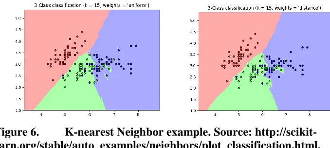
Figure 6. K-nearest Neighbor example. Source: http://scikit-learn.org/stable/auto_examples/neighbors/plot_classification.html. ... 26
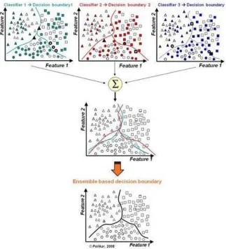
Figure 7. Pictorial Representation of how Ensemble works. Source: http://magizbox.com/training/machinelearning/site/ensemble/. ... 27
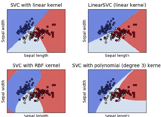
Figure 8. Pictorial representation of different kernels classification in SVM. Source: http://scikit-learn.org/stable/auto_examples/svm/plot_iris.html... 29
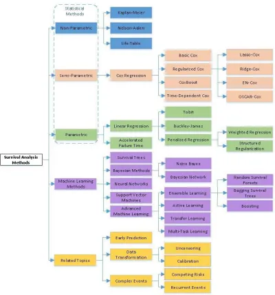
Figure 9. Taxonomy of methods developed for Survival Analysis. Image source: P. Wang et al. [41]... 31
Figure 10. Graphical representation of local clustering coefficient. Image source: Santillán et al. [35]. ... 42
Figure 11. An example of how PageRank is calculated. Image source: https://en.wikipedia.org/wiki/PageRank ... 43
Figure 12. Feature importance for the Facebook dataset. ... 50
Figure 13. Feature importance for the Wikipedia dataset. ... 50
xv
LIST OF ABBREVIATIONS BSU Boise State University
GC Graduate College
OSN Online Social Networks
RLTP Reciprocal Link Prediction problem AFT Accelerated Failure Time
BJ Buckley-James
Linear SVM Linear Support Vector Machine
SVM Support Vector Machine
RBF Radial Basis Function
SVR Support Vector Regression
AUC Area under Curve
AUROC Area under of ROC
TD-AUC Time Dependent AUC
KNN K-nearest Neighbors
CHAPTER 1: INTRODUCTION
Online social networks (OSN) have become popular among various age cohorts. People use them for not only socializing but also to gain insights on different day-to-day aspects, such as educational information, following the latest gossip, or interacting with peers around the clock. Some of these interactions can be Direct or Indirect. Direct Interaction is when a person/node exchanges information directly either through messages, emails, or calls, while the Indirect Interaction can be in many ways. People can have a third-party moderator to pass the word to connected family members and friends, or it can be strangers following up on a group conversation, and they help shape the social networks by creating new connections. While text messages and calls are traditional ways to interact, there are various forms of interactions on the Internet like Facebook’s wall posts, comments, likes, and shares, or Twitter’s tweets and re-tweets.
By Indirect Interaction between nodes 𝑢 and 𝑢, there is a particular action
depending on the type of network under study that involves both u and v (multiple times) during a given time interval [𝑢𝑢,𝑢𝑢). This study’s interest is in the Indirect Interactions between nodes that are not connected. Examples of Indirect Interactions are:
a) On social networks such as Facebook where users can interact with wall posts, comments, group conversations and information-sharing with users that are not on their friends’ list.
b) On Twitter, users can re-tweet or reply to tweets written by users who are not in their connections.
c) On the Wikipedia hyperlink network, readers can navigate from page 𝑢 to page 𝑢
through the search box (on the top right corner of page 𝑢) in case there is no explicit link on page 𝑢 to 𝑢. Some of these searches are casual and occasional, some last for a while because of current trending associations of topics, while others suggest the demand of a physical link from page 𝑢 to page 𝑢.
d) On the Amazon purchased products network, we can discover future co-purchased products by looking at users’ search logs that may suggest examples of product recommendations: people who purchased (or searched for) product 𝑢 may also be interested in product 𝑢. Moreover, when considering a pair of products, if there are a relatively higher number of users purchasing those two products, then it will be helpful to allocate them in some warehouses.
connections with others and share information. We can identify Indirect Interactions in such networks based on their common reviewed products and predict users’ future connections (friendships).
Indirect Interactions can be categorized as Dependent and
Figure 2. Indirect Interactions on Wikipedia. Source: https://en.wikipedia.org/wiki/Bollywood
The Indirect Interaction between nodes and during the time interval [𝑢𝑢,𝑢𝑢) is an indication that they may have something in common and is convenient to link them. However, not all Indirect Interactions are useful. Casual Indirect Interactions are irregular and may be “one-time” interactions among different nodes. For instance, on Wikipedia, during February 2016, when Donald Trump was nominated as Republican nominee, users navigated from his Wikipedia page to various other Wikipedia pages like Trump
University, Hollywood Walk of Fame, and Hillary Clinton. Though the number of
interactions between those pages was in the thousands, it was a casual interaction as it did not continue after that period.
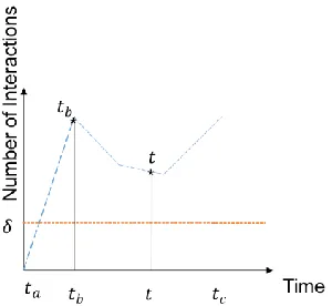
Persistent Indirect Interactions are indirect interactions that are continuous in a given time interval with interactivity always greater than a minimum threshold
irrespective of the presence of an edge between them.
Persistent Indirect Interactions: Let (𝑢,𝑢) be a pair of nodes having an Indirect
Interaction during the time interval [𝑢𝑢,𝑢𝑢). This Indirect Interaction is persistent during the time interval [𝑢𝑢,𝑢𝑢], if for each time 𝑢∈ [𝑢𝑢,𝑢𝑢], the number of Indirect
Figure 3. Persistent Indirect Interactions.
Persistent Interactions are the interactions that continue irrespective of an edge between them. Predicting connections can also be termed as Link Prediction but is different in a few aspects. Classical Link Prediction may or may not follow the interactivity between the pages, but it predicts future interactivity based on similarity. The scenarios below explain the Link Prediction on Wikipedia.
On Wikipedia, there were Indirect Interactions between two pages Doctor Strange
(film), and Baron Mordo in February 2016 and users continued to navigate between these two pages even until April 2016 with a threshold always higher than 10. Later on, in April 2016, an edge was created from Doctor Strange (film) to Baron Mordo.
Wikipedia is a vast network of new users and new links are added daily [14]. For such a network, editors manually check which of the Wikipedia pages need to have hyperlinks between them based on page content and thus add those new links to those sites. However, these hyperlinks are subject to change in the future. For example, there are links that are deleted after just two days of creation while some remain active. While some links are still unchanged, some are changed every day (like the Main_page [2] of Wikipedia where its content is updated every day). Oftentimes, there are a few links that exist for a long time, and they might never be used. Some of the existing statistics were given in [12] stating that out of 800,000 links added to the site in February, 66% of them were not even clicked or used once.
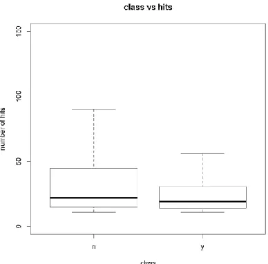
Figure 4. Box plot of hits concerning classes 𝒚 and 𝒏.
Figure 5. Histogram of hits density concerning classes 𝒚 and 𝒏.
The experimental results above also prove the same where class y define the existence of interactivity and class n define non-existence of interactivity.
other social networking sites like Twitter and Instagram. For all these suggestions, the only assumption is that they may know each other or may become future acquaintances. However, there is no guarantee that these users will have persistent interactions or no interaction at all. In such cases, these connections may not be useful.
In this thesis, when predicting links between a pair of nodes, priority is given to those links that will be useful in the future. On any social networking platform, it is better to recommend user 𝑢 to become friends with user 𝑢 if we know that these two nodes will interact in the future, rather than suggesting 𝑢́ as a friend for 𝑢 even after we know that 𝑢 and 𝑢́ will never interact. Thus, the longer the interaction is estimated to last between a pair of nodes; the higher is the priority for recommending a link between them.
Predicting connections in this study is different from the classical Link Prediction in the following ways:
I. Link Prediction aspects to predict links mostly by analyzing semantic similarities among the nodes. Whereas, the current study focuses on predicting connections based on Persistent Indirect Interactions.
II. Link Prediction focuses on growing the network by suggesting missing edges. However, it can sometimes lead to over-crowding by unused edges. This study focuses on predicting only such connections that are most likely to be useful in the future.
Wikipedia do not explain. Hence, the problem statement and the approach is to identify such Persistent Indirect Interactions and predict connections.
Two supervised learning approaches are proposed for the problem of predicting the Duration of Interactions. Given a set of network-based predictors, the basic approach consists of learning a binary classifier to predict whether or not an observed Indirect Interaction will last in the future. The second and more fine-grained approach consists of estimating how long the interaction will last by modeling the problem via Survival Analysis or as a Regression task. Once the duration is estimated, this information is leveraged for the Link Prediction problem.
An extensive experimental evaluation was performed with two longitudinal datasets, namely Facebook network and wall interactions, and Wikipedia Clickstream. This approach was tested to predict the Duration of Indirect Interaction and its
application to the Link Prediction task. Based on all the experiments, the results show that the more fine-grained approach (Survival Analysis on Facebook and Regression model on Wikipedia) has maximum improvement for predicting the Duration of Indirect Interactions and achieved an AUROC of 0.85 for Facebook and 0.77 on Wikipedia for Link Prediction. Moreover, this approach beats a Link Prediction model that does not consider the duration of interaction, is based only on network properties, and performs with an AUROC of 0.80 and 0.68 on Facebook and Wikipedia, respectively.
CHAPTER 2: RELATED WORK 2.1 Link Prediction
Link Prediction is a problem of predicting connections between two nodes in a network. This problem can be applied to different types of networks [21,22,23,24,25,53]. For comparatively small networks, it is possible to determine the links and add them to the network manually. However, due to the complexity and size of social networks, it is important to automate the process to reduce human intervention. Some of the notable types of approaches to tackle the Link Prediction problem are discussed next.
Liben-Nowell and Kleinberg [6] point out that social networks are highly
dynamic objects, new edges are added to the network along with the removal of some old (or) unused edges, from time to time. Their proposed work for the Link Prediction
problem uses a graph structure on five co-authorship networks available from the physics e-Print arXiv, www.arxiv.org. Some of the features introduced are the graph’s distance-based Common Neighbors, Jaccard’s coefficient, and Adamic/Adar features. One of the main problems of having these features on their dataset is that the pages of similar categories might have more neighbors in common, and hence have more leniency over predicting a hyperlink between those pages. While pages with a different set of neighbors belong to different categories, but are somehow related, might not have the same
future. Though the size of the dataset was small and it was during that time when the Link Prediction Problem was not yet addressed directly, they were able to explore the possible network and graph-based features. Their insights to those features are still used as baselines for most of the recent works. They address topological features like Shortest Distance, Clustering Index, some other Proximity features based on keyword match count, and Aggregated features like sum of neighbors, and the count of commonly published papers. Also, they give insight into the nature of different classifiers’
performances where SVM tend to have a good understanding and prediction over other classifiers.
Considering a network as a graph with nodes and edges, Grover, A., & Leskovec, J. [15] created an algorithm, ‘Node2Vec’, on multi-label classification and Link
Prediction problem that can be used on various real-world networks like Facebook or Protein-protein Interactions. It is a semi-supervised algorithm for scalable feature learning in networks. It is an optimized graph-based objective function to preserve neighborhood using random walks. Using the information from their algorithm, it is possible to understand and predict most probable labels of nodes in a network that are useful for Link Prediction. Depending on varying parameters in using Node2Vec (like the number of walks per node, context size, or the fraction of missing edges), it is possible to estimate node and edge features for any network in any domain. This algorithm can even be applied to an incomplete network with missing edges.
2.1.a Link Prediction on Wikipedia
However, Link Prediction does not entirely focus on Indirect Interactions; it involves other factors that can be helpful to predict future interactivity. There are many state-of-the-art works published based on the Link Prediction task. Some of the interesting related works on Wikipedia are discussed below.
Adafre et al. [5] proposed an approach to find missing links in the network by considering Wikipedia corpus and its underlying abstract words. They clustered all the Wikipedia pages to rank them by using LTRank and Lucene algorithms on the existing links to find similar pages. They stated that similar pages should have similar hyperlinks. They extracted anchor text from their related pages and predicted missing out-links in those similar pages. They then evaluated those missing links manually. Similar work was done by Noraset et al. [9] by considering text from Wikipedia pages. They proposed ‘3W’ to use semantic information of those pages and identify words/concepts to determine links to their referent pages.
obtain link candidates for the path. Based on those ranks, they were able to predict the top K pages for Link Prediction. Their evaluation was based on human raters available from Amazon Mechanical Turk (a platform where researchers post forms containing
questionnaire and participants get paid for each form response they give). Another such work by West et al. [11] is based on dimensionality reduction where they created an adjacency matrix based on out-links from a page 𝑢 to page 𝑢. They used principal component analysis on that matrix to determine which of those two pages should be linked. Their system was also evaluated using human raters’ responses on Amazon Mechanical Turk.
Paranjape et al. [12] constructed trees from the server logs of Wikipedia. These server logs consisted of information about each HTTP request from a user. The logs were grouped by user id, and most recent requests to a page were selected. On this available dataset, they used search proportion, path propagation, random walks and a combination of search and path propagation methods to identify potential link candidates. The number of page hits was the main component for three objective functions to list top K pairs of pages to be considered for a link between them. They tested their unsupervised results over editors’ choice of newly added links in the following month. Their results showed that most of the pairs predicted matched the editors’ choice of hyperlinks. This work is similar to the approach in this current thesis but is different in the following aspects:
of pairs from request logs. However, the pairs with counts less than ten are not included.
II. Their approach was to identify the top K pairs like (s, t) to place a link based on click-through rate which is the measure of times that users click on t given that they are in s. This current study’s approach focuses on determining Persistent
Indirect Interactions and suggest links based on users’ usage. Also, it does not solely rely on hit count but also on various other features as it was experimentally proven that hit counts do not effectively address a solution to the current problem. III. They used Search proportion, Path proportion, and Random walks to identify
potential pairs. This current study’s approach focuses only on the Search-based proportion, i.e. other pairs (see section 3.1) to determine Indirect Interactions. IV. Their work was validated with editors’ choice of links in the following months.
This current study’s approach is validated against the users’ choice of Persistent Interactions irrespective of a link.
2.2 Strength of Relationship
them because of the similarities among them.
There have been some interesting works published on estimating the strength of a relationship [19,35,36,37,38] in social networks like Twitter, Facebook, and Orkut. While some of the works focused on interaction, others focused on the connected network to identify string ties. Kumar et al.’s [20] study emphasizes on predicting edge weights to demonstrate the strength of their relationship. Zignani et al.’s [19] study was conducted to predict the strength of new links on the Facebook dataset. They re-used a dataset from [29] and tried to predict the strength of newly connected Facebook users. Their approach was to identify the strength of connection at the time of creation without the knowledge of prior interactions. They used temporal features to understand the interactivity.
Wilson et al. [36] addressed the issue of whether all the connections/links are valid indicators of real interactions among the users in a social network by performing experiments on 10 million crawled Facebook user profiles. They observed that the
interactivity on Facebook skewed towards a smaller portion of users’ friendship networks raising doubt as to whether or not all links imply equal friendship relationships. They also suggested that applications in social networks should consider interaction activity rather than mere connections.
Kahanda et al.’s [37] experimental findings indicate that it is necessary to consider transactional events such as file sharing, wall posts, photograph tags, and
messages as they are very useful for predicting link strength among the users in the social network. They also stated that while considering friendship, wall, picture and group attributes for the Facebook dataset, wall interactions had an utmost impact on their
the Twitter network based on historical interactivity. Their approach is to estimate the relationship strength between users [49, 50, 54, 55] based on direct interactions. Their framework included various graph-based, user-based and interaction-based features to fit their model.
Upon considering all the above-stated works, it is evident that for any social network, it is necessary to consider the interactivity to understand and perform any type of prediction tasks accurately and thus validating this current study’s approach.
2.3 Survival Analysis and Regression
Survival Analysis is a statistical measure to determine the probability that an event will occur. This current study estimates the duration of interaction between a pair of indirectly interacting nodes by using Survival Analysis to predict individual survival probabilities for an event (they will stop interacting), i.e., the probability that they will not stop interacting in the given period. Survival Analysis [40,57,64] (see section 4.2) is not only used in the medical domain to predict the probabilities for the occurrence of an event (i.e., chances or survival, estimated death probabilities), but also in generalizing an event and estimating its probability to occur. For example, Dave, V. S et al. [42] used Survival Analysis for the Reciprocal Link Prediction problem (RLTP). They used a cocktail Algorithm [40], and two other statistical survival methods Accelerated Failure Time (AFT) and Buckley-James (BJ) models along with Regression models like
Rakesh et al. [62] and Li et al. [63] used Survival Analysis on a Crowdfunding projects list. Crowdfunding is a platform for people to seek donations for completion of a project. It is an open platform where people can donate to a project of their interest. They studied whether the goal for the crowdfunding project was met within the stipulated time or not. While Rakesh et al. [62] examined the duration of successful projects by using censored regression models, Li et al. [63] also included the failed projects by using various logistic distributions.
Student retention rate is one of the major problems for a university. After
completing a semester, the rate of students who return to the same university to begin the next semester is called student retention rate. Student retention rate is important for a university to be ranked higher than other universities in a nation and also to secure government released funds. Survival Analysis was used on such data by Murtaugh et al. [59] and Ameri et al. [64] to estimate the time of event occurrence, i.e., whether a student will drop out or not and if so, when will they drop out.
CHAPTER 3: DATASETS
This study used two datasets to test Wikipedia Clickstream and Facebook network with wall interactions. The former is an example of a Node-Independent interactions’ network while the latter is an example of a Node-Dependent interactions’ network. Both datasets are discussed next.
3.1 Wikipedia Clickstream
Wikipedia Clickstream is Wikimedia’s research project in progress. It is a dataset consisting of pairs consisting of (referrer page, resource page) obtained from the
extracted request logs of Wikipedia. There are eight months of datasets released to date, starting from January 2015. Each dataset consists of four fields (Source: [1]).
1. prev: the result of mapping the referrer URL (or) Page title if it is on Wikipedia. 2. curr: the title of the webpage the client requested (or) Page title if it is on
Wikipedia.
3. type: describes (prev, curr)
a. link: if the referrer and request are both Wikipedia pages and the referrer links to the request;
b. external: if the referrer host is not en.wikipedia.org;
4. n: the number of occurrences (greater than 10) of the (referrer, resource) pair. Considered as the number of hits from prev to curr.
Thus far, the following datasets have been released for the English version of Wikipedia:
a) January 2015: This dataset includes columns of page ids for prev and curr. Redirects were not resolved.
b) February 2015: This dataset includes columns of page ids for prev and curr. Redirects were not resolved.
c) February 2016: More granular set of fixed values for hit counts.
d) March 2016: More granular set of fixed values for hit counts.
e) April 2016: There are three language versions of this dataset—Arabic, English, and Farsi. More granular set of fixed values is given in this dataset.
f) August 2016, September 2016, January 2017: These are latest versions released. For this study, February 2016, March 2016 and April 2016 are used as they are the longest consecutive months available in Clickstream.
3.1.a Estimating ground truth about duration of interactions
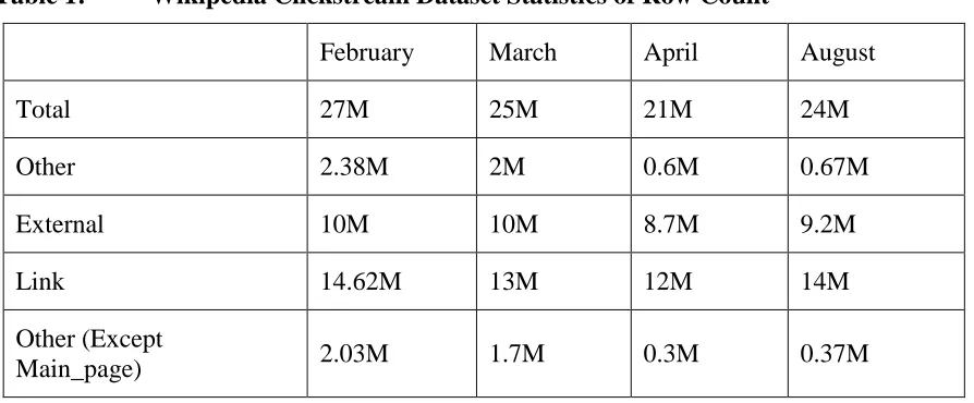
Table 1 gives an estimate of the total number of pairs for each type in each month. The Main_page is a recursively changing web page on Wikipedia. Though there are pairs with a considerably higher number of hit counts, they are considered as noise in the dataset. Hence, all the datasets are filtered to remove any occurrence of the Main_page among the pairs.
Table 1: Wikipedia Clickstream Dataset Statistics of Row Count
February March April August
Total 27M 25M 21M 24M
Other 2.38M 2M 0.6M 0.67M
External 10M 10M 8.7M 9.2M
Link 14.62M 13M 12M 14M
Other (Except
Main_page) 2.03M 1.7M 0.3M 0.37M
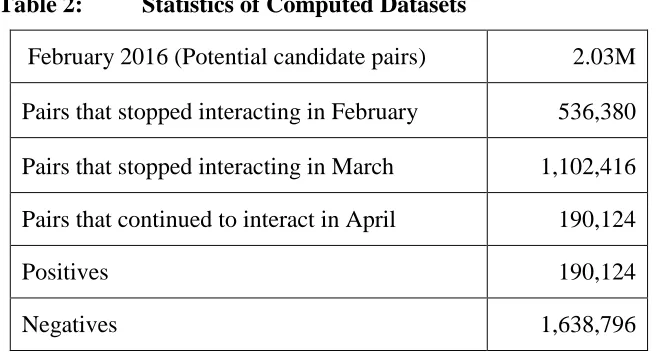
Table 2: Statistics of Computed Datasets
February 2016 (Potential candidate pairs) 2.03M Pairs that stopped interacting in February 536,380 Pairs that stopped interacting in March 1,102,416 Pairs that continued to interact in April 190,124
Positives 190,124
Negatives 1,638,796
3.2 Facebook
On Facebook, even though a pair of users may not be friends, they can still be part of a common activity. There are different types of interactions on Facebook through user’s wall posts, messages, comments, shares, and likes. Facebook wall interactions are when a user posts something on a friend’s timeline or vice versa that includes tagging. Interactions with the user’s friends list are Direct Interactions and interactions with public Facebook users or common friends with another user are called Indirect Interactions. The typical Indirect Interactions on Facebook include:
a) A mutual friend tagging two or more unconnected Facebook users in a single post.
b) Commenting on a common friend’s post.
c) Joining a common Facebook group and participating together by commenting on a post.
obtained data from September 2006 to January 2009. All the nodes and their information are anonymized. This dataset consists of information about:
a) Friendship (user1, user2, friendship creation timestamp)
b) Wall interactions (user1, user2, posts’ timestamp); where user2 is posting on
user1’s wall at a given timestamp.
Based on the availability of information in the dataset, only the interactions through wall posts are included in this current study.
3.2.a Estimating ground truth about duration of interactions
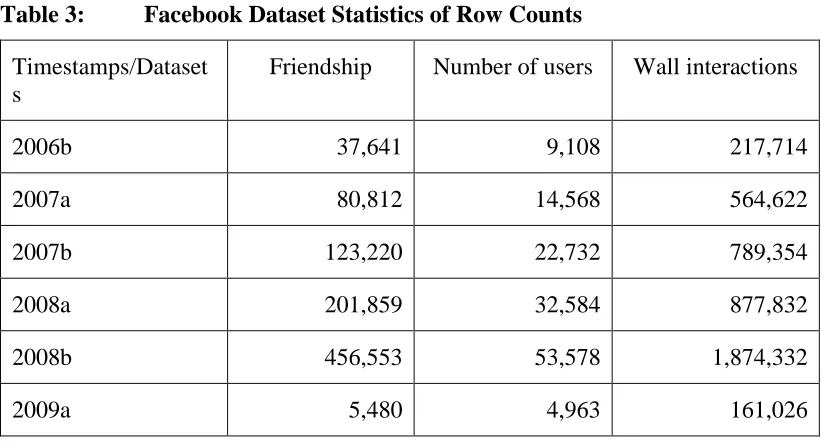
Table 3: Facebook Dataset Statistics of Row Counts
Timestamps/Dataset s
Friendship Number of users Wall interactions
2006b 37,641 9,108 217,714
2007a 80,812 14,568 564,622
2007b 123,220 22,732 789,354
2008a 201,859 32,584 877,832
2008b 456,553 53,578 1,874,332
2009a 5,480 4,963 161,026
With the similar approach followed for Wikipedia, we considered all the potential candidate pairs and determined which of those pairs stopped interacting or continued interacting in later months. The statistics of these results are given in Table 4. We considered the end time as the 2008b dataset and used the 2009a dataset for evaluation purposes. Hence, positives in this dataset for the classification approach are 88,155, and the negatives are 4,155.
Table 4: Facebook Dataset Final Statistics for Wall Interactions
Potential candidate pairs in 2006b 175,577
Pairs that stopped interacting in 2006b 88,155 Pairs that stopped interacting in 2007a 52,858 Pairs that stopped interacting in 2007b 21,399
Pairs that stopped interacting in 2008a 8,738
Pairs that stopped interacting in 2008b 4,155
CHAPTER 4: METHODS
Two supervised learning approaches are proposed to identify candidate pairs for Link Prediction. Given a set of network-based predictors, the basic approach consists of learning a binary classifier to predict whether or not an observed Indirect Interaction will last in the future. The second and more fine-grained approach consists of estimating how long the interaction will last by modeling the problem via Survival Analysis or as a Regression task. An outline of these methods is presented below.
4.1 Classification
Classification in Machine Learning is the categorization of data into different classes. There are different approaches and algorithms on how to classify based on the type of datasets (for example, documents can be classified based on content similarity). In machine learning, there are two different types of classifications—binary classification and multi-class classifications. Binary classification is the problem of having only two classes generally named as ′0′ or ′1′. The class ′0′ can also be defined as the classification of data into negatives (i.e., data does not belong to the desired class) and hence the class ′1′ can be defined as a classification of data into positives (i.e., data belongs to the desired class). Multi-class classification consists of more than two classes for the data to be classified. There are two learning approaches for classification: supervised and
predictability. The unsupervised learning model uses only unlabeled data to find underlying structures in the dataset. There are no metrics to evaluate the unsupervised learning models. Some of the supervised algorithms that were used for this thesis are: 4.1.a K-nearest Neighbors (KNN)
K-nearest neighbors (KNN) is a classification algorithm that uses distance or similarity for prediction. It places the tuples in the space to which they are closest to. Classification is done based on the majority vote of each nearest neighbors. For each class, there will be a query point that acts as a point of reference to calculate closeness. For the first iteration, a random data point is chosen as the query point and then
iteratively calculates query point until no other changes are possible. Figure 6 shows the distribution of points in a dataset with three classes and fifteen neighbors. The ‘weights’ parameter defines the value assigned on each data point. By default, it is ‘uniform’ and assigns equal weights to all data points. With weights= ‘distance,’ the classifier assigns weights inversely to each point regarding its distance to the query point.
4.1.b Random Forests
Random Forests is a type of an Ensemble model. The Ensemble model is a combination of more than one model. For example, in Figure 7, Classifier1 creates a decision boundary 1 to separate three shapes: circle, triangle, and square. It is not
accurate but works fine. Classifier 2 creates another decision boundary 2 and Classifier 3 creates decision boundary 3. An ensemble model formed by combining all the three classifiers gave an accurate decision boundary to separate shapes effectively.
Random Forests is one such model that uses an ensemble of randomly generated trees on various subsets of the dataset. It uses averaging to improve accuracy and also controls the problem of over-fitting.
4.1.c Logistic Regression
Logistic Regression gives the probabilistic view of Regression [65]. Assuming a binary class, and 𝑢 as the vector of features for the classifier, then logistic regression finds the probability 𝑢 that the class belongs to class ′1′ then the probability is given by
𝑢= 1 𝑢−𝑢𝑢+1
where 𝑢 is a vector of constants.
It is also a supervised learning model with different algorithms like the liblinear, newton-cg, or saga. This current study used the liblinear algorithm.
4.1.d Support Vector Machines
Figure 8. Pictorial representation of different kernels classification in SVM. Source: http://scikit-learn.org/stable/auto_examples/svm/plot_iris.html.
4.2 Survival Analysis
Estimating the duration of an event to occur is one of the critical problems in
analyzing data. It is possible that during any study on a group of entities, there might be instances for which the event did not occur within the study’s duration or may have incomplete, missing, or unavailable data about the event occurrence. Such instances are called censored instances that can be effectively approached using Survival Analysis [40, 41, 55, 58, 59]. Survival Analysis uses hazard functions which determines the rate of occurrence of an event at a time t with the condition that the event did not happen before time t. The results of this function are applied to different statistical methods of Survival Analysis to estimate the final probabilities for each of the entities. The following
a) Non-parametric: Specific methods of this type are Kaplan-Meir, Nelson-Aalen, and Life-Table. These methods are mainly used when there no theoretical distribution of the event occurrences are known.
b) Semi-parametric: Specific methods of this type are the Cox model, Regularized Cox, CoxBoost and Time-Dependent Cox. These methods are mainly used where the knowledge about the distribution of survival times are not necessary.
c) Parametric: Specific methods of this type are Tobit, Buckley-James, Penalized Regression and Accelerated failure Time. These methods are mainly used when the patterns in survival times distribution are known.
d) Machine Learning methods: There are Survival trees, Bayesian methods, and Neural networks.
Figure 9 illustrates various Survival Analysis methods.
Figure 9. Taxonomy of methods developed for Survival Analysis. Image source: P. Wang et al. [41]
4.3 Regression
In statistical analysis, regression is a process of estimating the relationships among variables, such as a regression model for variable 𝑢 with respect for feature vector variable 𝑢 and a constant vector 𝑢. i.e.,
CHAPTER 5: APPROACH
In this chapter, we propose approaches to the problem of predicting how long an Indirect Interaction between two nodes will last. The Indirect Interaction on Facebook is about a pair of unconnected users participating in a common interaction like comments, group messages, shares, and wall posts. Similarly, on Wikipedia, Indirect Interaction is between two pages where users navigate through the search box. This study examines the cases that involved multiple interactions between 𝑢 and 𝑢 during an observational time interval [𝑢𝑢,𝑢𝑢]. The Indirect Interaction between nodes 𝑢 and 𝑢 during that time interval indicates that 𝑢 and 𝑢 may have something in common, and it might be useful to link them.
Problem Definition: Given two nodes 𝑢 and 𝑢 in a network such that during the
time interval [𝑢𝑢,𝑢𝑢)
(1) there is no link between them, and
(2) we observe an “Indirect Interaction” between 𝑢 and 𝑢
predict how long the nodes 𝑢 and 𝑢 will keep interacting after 𝑢𝑢.
This problem has applications in link recommendation. When recommending a link
between two nodes 𝑢 and 𝑢, we prefer to recommend links that will be useful in the
future. In fact, in any social networking platform, it is better to recommend user 𝑢 to
rather than suggesting 𝑢́ as a friend for 𝑢 even after we know that 𝑢 and 𝑢́ will never interact.
Thus, the longer the interaction is estimated to last between a pair of nodes; the
higher the priority is for recommending a link between them.
In our framework, we consider the time period divided into the following intervals:
a) [𝑢𝑢,𝑢𝑢) is the time interval used to observe Indirect Interactions between nodes;
b) [𝑢𝑢,𝑢𝑢] is the time interval used to observe when the Indirect Interaction(s) will
stop;
c) (𝑢𝑢,𝑢𝑢] is the time interval used to observe which links have been formed.
We propose two supervised learning approaches to the problem of predicting the duration of Indirect Interaction. Given a candidate pair of indirectly interacting nodes 𝑢= (𝑢,𝑢) and a vector of network-based predictors 𝑢𝑢, the basic approach consists of
predicting whether or not the Indirect Interaction 𝑢= (𝑢,𝑢) will last, while the more fine-grained approach consists of estimating how long the Indirect Interaction will last. These approaches are detailed in the following sections.
5.1 Basic Approach
In order to predict whether the Indirect Interaction between a pair of non-linked
nodes 𝑢= (𝑢,𝑢) will last or not, we model the problem as a binary classification task
where the input features are given by 𝑢𝑢and the positive class is given by the set of
instances that do not stop interacting in the time interval [𝑢𝑢,𝑢𝑢], i.e., their Indirect
time 𝑢𝑢 ≤ 𝑢≤𝑢𝑢fall into the negative class.
5.2 Fine-grained Approach
To predict the Indirect Interaction duration in the time interval [𝑢𝑢,𝑢𝑢], two
different methods were used—Survival Analysis and Regression. Next, we describe how
we model the problem according to these two methods.
5.2.a Modeling the Problem via Survival Analysis
Survival Analysis is a statistical method to estimate the expected duration of time
until an event of interest occurs [41].
We apply Survival Analysis to the interval [𝑢𝑢,𝑢𝑢] to compute the survival time
of an Indirect Interaction. The event of interest is when the Indirect Interaction between two nodes stops. The time when the event of interest happens for the instance 𝑢= (𝑢,𝑢) is denoted by 𝑢𝑢. During the study of our Survival Analysis problem, it is possible that the event of interest was not observed for some instances. This occurs because we are observing the problem in a limited time window [𝑢𝑢,𝑢𝑢] or we missed the traces of some instances. If this happens for an instance 𝑢 we say that 𝑢 is censored and denote by 𝑢𝑢 the censored time. Given an instance 𝑢, we denote by 𝑢𝑢 the feature vector. Let 𝑢𝑢 be
a Boolean variable indicating whether or not the instance 𝑢 is not censored, i.e., if 𝑢𝑢 =
1 then the instance 𝑢 is not censored. We denote by 𝑢𝑢 the observed time for the
instance 𝑢 that is equal to 𝑢𝑢 if 𝑢 is uncensored and 𝑢𝑢 otherwise.
𝑢𝑢 = { 𝑢𝑢 𝑢𝑢 𝑢𝑢 =1 𝑢𝑢 𝑢𝑢 𝑢𝑢 =0
Given a new instance 𝑢 described by the feature vector 𝑢𝑢, Survival Analysis
estimates a survival function 𝑢𝑢 that gives the probability that the event for the instance
𝑢𝑢(𝑢) =𝑢𝑢 (𝑢𝑢≥ 𝑢)
The survival function can be used to compute the expected time 𝑢̂𝑢of event
occurrence for an instance 𝑢 as explained in the next section. 5.2.b Modeling the Problem via Regression
Another way to estimate the duration of an Indirect Interaction is to model the problem as a Regression task, i.e., estimating the parameters 𝑢 of a function 𝑢 such that 𝑢𝑢 ≈𝑢(𝑢,𝑢), for each instance 𝑢 in the training set.
The main difference between Regression and Survival Analysis is that regression is not able to incorporate the information coming from censored instances within the predictive model. In the case of regression, censored instances are typically ignored or their observed time 𝑢 is modeled as constant 𝑢𝑢 much bigger than 𝑢𝑢.
5.3 Link Prediction
In this section, we address the problem of predicting whether or not a pair of non-linked nodes showing an Indirect Interaction will become a link in the future. We adopt the Link Prediction framework with a single feature proposed by Liben-Nowell and Kleinberg [6]. This framework consists of the following steps:
a) assign a score to each candidate pair of non-linked nodes,
b) order the candidate pairs in descending order and take the top-n pairs with the highest score,
c) evaluate how many of these top-n pairs are links in the test set.
are predicted to last a shorter time because in the former case linking the two nodes can be more beneficial for both of them. Therefore, we propose to assign 𝑢𝑢𝑢𝑢𝑢 (𝑢,𝑢) to each pair of indirectly interacting nodes (𝑢,𝑢) that are not linked during the time interval [𝑢𝑢,𝑢𝑢) that is proportional to the estimated duration of their Indirect Interaction during
the time interval [𝑢𝑢,𝑢𝑢]. As we proposed various methods in the previous section to
predict the Indirect Interaction duration, the value of 𝑢𝑢𝑢𝑢𝑢 (𝑢,𝑢) depends on the method used.
5.3.a Classification
When using classification, 𝑢𝑢𝑢𝑢𝑢 (𝑢,𝑢) is equal to the probability given by the classifier that the instance 𝑢= (𝑢,𝑢) is in the positive class, i.e., the Indirect Interaction will last.
5.3.b Survival Analysis
When using Survival Analysis, the score is given by the expected time 𝑢̂𝑢 the interaction is predicted to stop, i.e. 𝑢𝑢𝑢𝑢𝑢 (𝑢,𝑢) =𝑢̂𝑢. The predicted expected time 𝑢̂𝑢
of event occurrence is computed as follows. From the Survival Analysis model, we will have the following probabilities:
𝑢𝑢(𝑢𝑢) =𝑢𝑢 (𝑢𝑢 ≥𝑢𝑢), 𝑢𝑢(𝑢𝑢+1) =𝑢𝑢 (𝑢𝑢 ≥𝑢𝑢+1), …, 𝑢𝑢(𝑢𝑢) =
𝑢𝑢 (𝑢𝑢 ≥ 𝑢𝑢). The probability 𝑢𝑢 (𝑢𝑢+𝑢≤ 𝑢𝑢 ≤𝑢𝑢+𝑢+1), that the Indirect
Interaction will stop in the interval [𝑢𝑢+𝑢,𝑢𝑢+𝑢+1) is given by
𝑢𝑢 (𝑢𝑢+𝑢≤𝑢𝑢 ≤𝑢𝑢+𝑢+1) =𝑢𝑢 (𝑢𝑢 ≥𝑢𝑢+𝑢) −𝑢𝑢 (𝑢𝑢 ≥𝑢𝑢+𝑢+
1)
for 0≤ 𝑢< 𝑢, where 𝑢 is the number of units we divided the interval [𝑢𝑢,𝑢𝑢] into.
𝑢̂ = (∑𝑢 𝑢𝑢=1 (𝑢+1) ×𝑢𝑢 (𝑢𝑢+𝑢≤𝑢𝑢 ≤ 𝑢𝑢+𝑢+1) ) + (𝑢×𝑢𝑢 (𝑢𝑢 ≥
𝑢𝑢) )
Because we have a limited time window [𝑢𝑢,𝑢𝑢] to observe when the Indirect Interaction is stopping, when 𝑢̂ = 𝑢 𝑢𝑢 we have a lower bound on when the interaction is
stopped, i.e., the Interaction can stop at any time 𝑢≥𝑢𝑢 , but we do not know exactly when.
5.3.c Regression
When using Regression, 𝑢𝑢𝑢𝑢𝑢 (𝑢,𝑢) =𝑢̂𝑢 where 𝑢̂ ≈𝑢 𝑢(𝑢,𝑢) is the
CHAPTER 6: LIST OF PREDICTORS
In this chapter, we report the set of predictors used in our thesis. The predictors are computed by considering the network [34] and are divided into three types of features namely Node-based features, Neighborhood-based features, and Network-based features. Additionally, some extra features on page content are used based on the availability of resources (Wikipedia API - sandbox) to gather such information.
6.1 Notations in Formulae:
Let 𝑢= (𝑢,𝑢: 𝑢) be an undirected weighted graph where
a) 𝑢is a set of vertices and
b) 𝑢⊆𝑢×𝑢 is the set of Edge(s)
c) 𝑢:𝑢→𝑍+
Let u be a node in 𝑢, we denote by 𝑢(𝑢) is the set of neighbors of node 𝑢 where
𝑢(𝑢) = {𝑢∈ 𝑢| (𝑢,𝑢) ∈𝑢 ⋁ (𝑢,𝑢) ∈𝑢 }
For directed graphs, we define 𝑢𝑢𝑢(𝑢) to be the set of neighbors pointed towards 𝑢, i.e.,
6.2 Node-based features
6.2.a Degree
For an undirected graph, the number of edges that connects a node with its neighbors is called Degree [44] of that node, denoted by
𝑢𝑢𝑢 (𝑢) = |𝑢(𝑢)|
For directed graphs, we consider In-degree and Out-degree denoted by 𝑢𝑢𝑢𝑢𝑢 and 𝑢𝑢𝑢𝑢𝑢𝑢 respectively, where
𝑢𝑢𝑢𝑢𝑢 (𝑢) = |𝑢𝑢𝑢(𝑢)|
and 𝑢𝑢𝑢𝑢𝑢𝑢 (𝑢) = |𝑢𝑢𝑢𝑢(𝑢)| 6.2.b Reciprocity
For a directed graph with 𝑢,𝑢 as nodes, if 𝑢 has an edge to 𝑢, reciprocity is to identify if there was an edge from 𝑢 to 𝑢. The weights on such edges are used as one of the predictors, i.e.,
𝑢𝑢𝑢(𝑢,𝑢) =𝑢(𝑢,𝑢)
6.3 Neighborhood-based features
6.3.a Common-Neighbors (CN)
Common Neighbors between nodes 𝑢 and 𝑢 is the number of nodes that have a common edge with both nodes 𝑢 and 𝑢. As stated in [6,16,20,21,23], common neighbor is a state-of-the-art measure that can be applied to any network to understand the
popularity of the pair of nodes. Common neighbors is given by the following formula. 𝑢𝑢(𝑢,𝑢) = |𝑢(𝑢) ∩𝑢(𝑢)|, if the graph is undirected.
6.3.b Jaccard similarity
It is a measure mainly used to compute similarity and diversity of the two nodes. If 𝑢and 𝑢 are two nodes in a network, Jaccard similarity [6,16] is measured as the intersection of neighbors between u and v over union of their neighbors. Hence, it is given by the following formula for undirected graphs
𝑢𝑢𝑢(𝑢,𝑢) =|𝑢(𝑢) ∩𝑢(𝑢)| |𝑢(𝑢) ∪𝑢(𝑢)|
and for directed graphs,
𝑢𝑢𝑢(𝑢,𝑢) =|(𝑢𝑢𝑢(𝑢) ∪𝑢𝑢𝑢𝑢(𝑢)) ∩ (𝑢𝑢𝑢(𝑢) ∪𝑢𝑢𝑢𝑢(𝑢))| |(𝑢𝑢𝑢(𝑢) ∪𝑢𝑢𝑢𝑢(𝑢)) ∪ (𝑢𝑢𝑢(𝑢) ∪𝑢𝑢𝑢𝑢(𝑢))|
6.3.c Adamic-Adar similarity
It is a similarity measure that weights common neighbors with few connections more heavily. It ensures to prioritize the least connected common neighbor.
Mathematically, Adamic-Adar [4] is the sum of the inverse log of the count of neighbors of all the common neighbors between u and v.
𝑢𝑢(𝑢,𝑢) = ∑
𝑢∈𝑢(𝑢)∩𝑢(𝑢)
1 𝑢𝑢𝑢|𝑢(𝑢)|
6.3.d Preferential Attachment score
The preferential attachment score is an aggregated neighborhood-size based feature. For this study, degree(s) are aggregated as preferential attachment score [16] and is given by
𝑢𝑢(𝑢,𝑢) = |𝑢(𝑢)| × |𝑢(𝑢)| for undirected graphs.
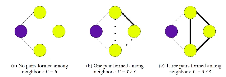
6.3.e Local Clustering Coefficient
Local Clustering coefficient [16] is the property of a node within the network. If 𝑢 is a node, the number of triangles formed using its neighbors with respect to number of
its neighbors is the local clustering coefficient. It is the probability that the neighbors of the node are connected.
𝑢(𝑢) = 2×|{𝑢1,𝑢2 ∈𝑢(𝑢)}|
|𝑢(𝑢)|×(|𝑢(𝑢)|−1)
Figure 10 shows an example for computing local clustering coefficient in a sample network.
Figure 10. Graphical representation of local clustering coefficient. Image source: Santillán et al. [35].
6.4 Network-based features
6.4.a PageRank
𝑢𝑢(𝑢) =1−𝑢
|𝑢| + 𝑢∑𝑢∈𝑢𝑢𝑢(𝑢)
𝑢𝑢(𝑢) |𝑢𝑢𝑢𝑢(𝑢)| where d is the dumping factor usually set to 0.85.
Figure 11 shows an example of PageRank for all nodes in an example network.
Figure 11. An example of how PageRank is calculated. Image source: https://en.wikipedia.org/wiki/PageRank
6.4.b Node2Vec
Deepwalk (Perozzi et al. [46]), and Spectral Clustering (Tang et al. [48]) in the task of node Link Prediction. Node2Vec is an embedding technique based on random walks. It computes the embedding in two steps. First, the context of a node (or neighborhood at distance 𝑢) is approximated with biased random walks of length 𝑢 that provides a trade-off between breadth-first and depth-first graph searches. Second, the values of the embedding features for the node are computed by maximizing the likelihood of generating the context by the given node. Node2Vec uses only the structure of the network and does not consider any node or edge label.
As the node features are computed for each in pair (𝑢,𝑢), edge features can be learned with a choice of any below binary operator on those node features. For 𝑢 and 𝑢 nodes, 𝑢𝑢(𝑢) and 𝑢𝑢(𝑢) are their respective Node2Vec features.
a) Adamard: (𝑢𝑢(𝑢)+2𝑢𝑢(𝑢))
b) Hadamard: (𝑢𝑢(𝑢) ×𝑢𝑢(𝑢))
c) Weighted-L1: |𝑢𝑢(𝑢) −𝑢𝑢(𝑢)|
d) Weighted-L2: : |𝑢𝑢(𝑢) −𝑢𝑢(𝑢)|2
The Hadamard was used in this study for learning edge features as it was shown to perform best by Grover and Leskovec [15]. Regarding the significance of weights on the edges, we used hits as weights on the network [20]. We used 40 dimensions with six walk-length, and variable 𝑢 set to 0.3 as parameters for the Node2Vec algorithm.
6.5 Additional Wikipedia Page features
of additional features can be included in the dataset. However, for Facebook, as the data is anonymized, it is difficult to retrieve individual node properties like content from their wall posts, comments or any other information that can help to identify additional
node/edge properties. 6.5.a Categories’ similarity
Each Wikipedia page falls under a set of categories. As an example, the page ‘Niagara Falls’ falls under the set of categories Waterfalls of Ontario, Block waterfalls, Waterfalls of New York, and so forth. Thus, pages with more categorical similarities may have some relatedness between them [18]. Let 𝑢 and 𝑢 be Wikipedia pages; we define 𝑢𝑢𝑢(𝑢) as the set of categories of page 𝑢 and 𝑢𝑢𝑢𝑢𝑢(𝑢) as the set of pages that belong
to category 𝑢. Then we defined categories’ similarity for a pair of pages 𝑢 and 𝑢 in terms of:
a) the Jaccard similarity between the pages’ categories as
𝑢𝑢𝑢𝑢𝑢𝑢(𝑢,𝑢) =|𝑢𝑢𝑢(𝑢) ∩𝑢𝑢𝑢(𝑢)| |𝑢𝑢𝑢(𝑢) ∪𝑢𝑢𝑢(𝑢)|
b) the Adamic-Adar similarity as
𝑢𝑢𝑢𝑢𝑢(𝑢,𝑢) = ∑
𝑢∈𝑢𝑢𝑢(𝑢)∩𝑢𝑢𝑢(𝑢)
1
𝑢𝑢𝑢 |𝑢𝑢𝑢𝑢𝑢(𝑢)|
c) the Preferential Attachment score on pages’ categories as
CHAPTER 7: EXPERIMENTS
As explained in the framework for our approach, we distributed each of the
datasets into three time periods. The time periods were set as follows:
a) for Facebook, we set 𝑢𝑢 = September 2006, 𝑢𝑢 = January 2007, 𝑢𝑢 = 𝑢𝑢 = December 2008, and 𝑢𝑢 = January 2009;
b) for Wikipedia, we set 𝑢𝑢 = February 2016, 𝑢𝑢 = March 2016, 𝑢𝑢 = April 2016, 𝑢𝑢 = July 2016 and 𝑢𝑢 = August 2016.
For each dataset, we selected all pairs of nodes I that showed Indirect Interaction(s) in the time interval [𝑢𝑢,𝑢𝑢). Then, for each pair 𝑢= (𝑢,𝑢) ∈𝑢, we
checked whether (𝑢,𝑢) continued to interact in the interval persistently. If not, we set 𝑢𝑢 =0, if yes, then 𝑢𝑢 was set to the time 𝑢∈ [𝑢𝑢,𝑢𝑢] when the persistent interaction
stopped, and if the persistent interaction never stopped in the interval [𝑢𝑢,𝑢𝑢], we
considered the instance 𝑢 to be censored. The number of instances of nodes with Indirect Interactions and the number of censored instances is reported for each dataset in Table 5. For Wikipedia, we filtered other types of tuples having prev or curr page title as
In all the datasets, we considered the class imbalance problem (i.e., we have more negative instances (instances that stopped interacting anytime 𝑢∈ [𝑢𝑢,𝑢𝑢]than positive
instances (instances that did not stop interacting in the observational period); these are censored instances). We used a majority under sampling strategy for a similar problem [42]. For each dataset, we created a pool of sub-datasets. First, we created ten random samples of the majority class whose size is set to be the same as one of the minority class. Then, we added each of these samples to all the instances in the minority class and
performed a five-fold cross-validation on each of those ten balanced datasets. We finally averaged the results obtained from all the five-fold cross-validated datasets. We used the same subsets of datasets across all the experiments.
Table 5: Indirect Interactions
Dataset Instances of Indirect Interactions Censored Instances
Facebook 175,577 4,155
Wikipedia 2.03M 190,124
7.1 Predicting Duration of Indirect Interactions
The first problem studied in this thesis was to estimate the duration of interactions in each of the datasets. This problem was addressed in two ways. First, the binary
classification approach was used to determine whether or not they will continue to interact at time 𝑢𝑢. Second, the more fine-grained approach was used to estimate the duration of interactions using Survival Analysis and Regression.
7.1.a Will the Indirect Interactions last or not?
predict whether the Indirect Interactions would last or not. In this case, we considered
censored instances as positive instances (i.e., to say that the interaction will last) and
instances where the event occurred (i.e., they stopped interacting) as negative instances.
For each dataset, using all the listed predictors, five classification models are used to determine the best fit model in predicting whether or not they will continue to interact at time 𝑢𝑢. Table 6 below shows the results obtained using the following
classifiers.
1. K-nearest neighbors with number of neighbors set as 5. 2. Random Forests with 100 trees and criterion set as “entropy.” 3. Linear-Support Vector Machine with a maximum of 100 iterations. 4. Radial Basis Function (RBF) kernel of SVM.
5. Linear model’s Logistic Regression. Table 6: Results from Classifiers - Facebook
Classifier Accuracy AUROC MAP Precision
(class1)
Precision (class0)
KNN 0.603 0.633 0.648 0.610 0.597
Linear SVM 0.680 0.743 0.751 0.734 0.646
Logistic Regression 0.677 0.737 0.746 0.715 0.651
Random Forests 0.832 0.901 0.894 0.808 0.861
SVM_RBF 0.500 0.505 0.598 0.541 0.468
same parameters on the classifiers for experiments on the Wikipedia dataset, Table 7 shows the results obtained.
Table 7: Results from Classifiers - Wikipedia
Classifier Accuracy AUROC MAP Precision
(class1)
Precision (class0)
KNN 0.668 0.720 0.732 0.671 0.664
Linear SVM 0.631 0.689 0.693 0.674 0.605
Logistic Regression 0.634 0.694 0.703 0.678 0.607
Random Forests 0.712 0.783 0.785 0.730 0.697
SVM_RBF 0.499 0.507 0.549 0.416 0.495
The classifier with the best performance is Random Forests with an AUROC of 78.3%. Tables 6 and 7 show results by using similar features in both datasets. However, by including additional categorical features on the Wikipedia Dataset, the following results are observed.
Table 8: Results from Classifiers including Categorical Features - Wikipedia
Classifier Accuracy AUROC MAP Precision
(class1)
Precision (class0)
KNN 0.697 0.761 0.762 0.698 0.696
Linear SVM 0.659 0.731 0.726 0.742 0.619
Logistic Regression 0.670 0.730 0.732 0.692 0.663
Random Forests 0.747 0.834 0.825 0.743 0.752
The classifier with the best performance is Random Forests with an AUROC of 83.4% and is higher than the previously achieved AUROC of 78.3%. From the results above, it is evident that inclusion of available categorical features improved the system’s performance.
7.1.b Feature Importance
Of all the predictors used for the approach, we measured the importance of each predictor to understand their contribution towards the performance of the approach. The following figures compare the ‘feature importance’ for each of the predictors.
Figure 12. Feature importance for the Facebook dataset.
Figure 13. Feature importance for the Wikipedia dataset.
they are denoted by prev and curr. Also, ‘CN’ denotes Common Neighbors, ‘PG’ denotes
PageRank, ‘weight’ is the reciprocal edge weight and ‘recip’ is Reciprocity of the edge. As we can see in the figures, the highest important features vary for different datasets. There is no concrete notion as to which of these predictors are commonly important for any dataset.
Figure 14. Feature importance for Wikipedia dataset (with Categorical features).
Figure 14 shows the order of important features for the Wikipedia dataset including additional categorical features. It is evident that these additional features contribute comparatively higher towards better performance.
7.1.c Comparison of Classification with Baselines
Some of the important predictors that are capable of predicting independently are Hits, Jaccard similarity score, Adamic-Adar similarity score, Preferential Attachment score and Node2Vec features. As we had evaluated 40 Node2Vec features for each node, we calculated Cosine similarity of those node features to construct it in a single column. These predictors are scores evaluated on pairs (𝑢,𝑢) together. To effectively determine the performance of our proposed system, it was necessary to compare and understand if it could perform better than the baselines. We used the following features to compare:
2. Adamic-Adar similarity score 3. Preferential Attachment score
4. Cosine similarity of Node2Vec node features. 5. Hit counts
Only the above-stated features were chosen as they determine the feature of (𝑢,𝑢) together in a network. Table 9 and 10 show baselines’ results for both the datasets.
Table 9: Results for Baselines - Facebook
Baselines AUROC MAP
Hits 0.633 0.693
Jaccard Similarity 0.707 0.701
Adamic Adar Similarity 0.292 0.386
Preferential Attachment 0.612 0.624
Node2Vec 0.576 0.579
Table 10: Results for Baselines - Wikipedia
Baselines AUROC MAP
Hits 0.455 0.459
Jaccard Similarity 0.556 0.556
Adamic Adar Similarity 0.573 0.611
Preferential Attachment 0.572 0.591
Node2Vec 0.583 0.570
7.1.d How long will the Indirect Interaction last?
interacting at time 𝑢𝑢.” We then used the predicted probability to calculate the Survival
Function values. For each pair of nodes in the datasets, we calculated the expected value of survival probabilities, i.e., 𝑢(𝑢,𝑢). In Survival Analysis, we used the Accelerated Failure Time (AFT) model with five distributions, and three Regression models:
1. For AFT: a. Weibull b. LogNormal c. Exponential d. Cox
2. Regression:
a. Ridge Regression b. Lasso Regression
c. Support Vector Regression (SVR) using ‘rbf’ kernel
As these datasets have censored information; classical AUROC is not suitable. To compare the performances of these two sets of algorithms, we considered two metrics that are commonly used to evaluate Survival Analysis models, namely c-index and Mean Absolute Error (MAE) [41]. The c-index is given by the formula:
𝑢−𝑢𝑢𝑢𝑢𝑢 = 1
𝑢𝑢𝑢𝑢𝑢∑
:𝑢𝑢=1
∑
𝑢𝑢>𝑢𝑢
1(𝑢̂𝑢> 𝑢̂𝑢)
where 𝑢𝑢𝑢𝑢 is the number of all pairs (𝑢𝑢,𝑢𝑢) such that 𝑢𝑢 =1 (non-censored