Hydrographic Surface Modeling Through A Raster Based Spline Creation Method

University of New Orleans University of New Orleans

ScholarWorks@UNO

ScholarWorks@UNO

University of New Orleans Theses and

Dissertations Dissertations and Theses

Spring 5-16-2014

Hydrographic Surface Modeling Through A Raster Based Spline

Hydrographic Surface Modeling Through A Raster Based Spline

Creation Method

Creation Method

Julie G. Alexander

University of New Orleans, [email protected]

Follow this and additional works at: https://scholarworks.uno.edu/td

Part of the Databases and Information Systems Commons, Graphics and Human Computer Interfaces Commons, and the Numerical Analysis and Scientific Computing Commons

Recommended Citation Recommended Citation

Alexander, Julie G., "Hydrographic Surface Modeling Through A Raster Based Spline Creation Method" (2014). University of New Orleans Theses and Dissertations. 1842.

https://scholarworks.uno.edu/td/1842

This Thesis-Restricted is protected by copyright and/or related rights. It has been brought to you by

ScholarWorks@UNO with permission from the rights-holder(s). You are free to use this Thesis-Restricted in any way that is permitted by the copyright and related rights legislation that applies to your use. For other uses you need to obtain permission from the rights-holder(s) directly, unless additional rights are indicated by a Creative Commons license in the record and/or on the work itself.

Hydrographic Surface Modeling Through A Raster Based Spline Creation Method

A Thesis

Submitted to the Graduate Faculty of the University of New Orleans in partial fulfillment of the requirements for the degree of

Master of Science in

Computer Science

by

Julie Alexander

A.S. Mississippi Gulf Coast Community College 2009 B.S. Computer Science University of Southern Mississippi 2011

Acknowledgements

Table of Contents

Abstract ... iii

List of Figures ...v

1 Introduction ...1

2 Background ...4

2.1 Surveying Methods ...4

2.2 Digital Survey Data...7

3 Model Development Algorithms ...9

3.1 Current Modeling Techniques ...9

3.2 The Hydraulic Spline Algorithm ...13

3.3 Comparative Advantages of Raster Data in Geospatial Applications ...19

3.4 A Raster based Hydraulic Spline Method ...20

4 Implementation ...25

4.1 Oracle Data Storage ...25

4.2 Methodology ...28

4.3 Challenges ...45

5 Conclusion ...47

5.1 Possible Applications ...47

5.2 Future Work ...48

5.3 Summary ...49

6 Bibliography ...51

7 Appendix ...53

Abstract

The United States Army Corp of Engineers relies on accurate and detailed surface models for

various construction projects and preventative measures. To aid in these efforts, it is necessary to

work for advancements in surface model creation. Current methods for model creation include

Delaunay triangulation, raster grid interpolation, and Hydraulic Spline grid generation. While

these methods produce adequate surface models, attempts for improved methods can still be

made.

A method for raster based spline creation is presented as a variation of the Hydraulic Spline

algorithm. By implementing Hydraulic Splines in raster data instead of vector data, the model

creation process is streamlined. This method is shown to be more efficient and less

computationally expensive than previous methods of surface model creation due to the inherent

advantages of raster data over vector data.

List of Figures

Figure 2.1 A graphical representation of a profile (shown as a dashed line) and its corresponding

center lines (shown as solid lines).

Figure 2.2: LiDAR Image – FEMA LiDAR Dataset Louisiana 2006

Figure 3.1: Merged surface point data

Figure 3.2: A surface raster generated using an inverse distance weighted function

Figure 3.3: Setting up the Hydraulic Spline Algorithm

Figure 3.4: Spline Set up

Figure 3.5: Supplementing the Centerline (Profile)

Figure 3.6: Evaluating splines for the creation of polygons

Figure 3.7: A graphical representation of mesh generation

Figure 3.8: A representation of selecting profile cross section intersecting pixels in raster data

Figure 3.9: Algorithm 1: Setting up splines in raster space

Figure 3.10: Supplementing the center line

Figure 3.11: Algorithm 2: Supplementing the centerline

Figure 3.12: The bounding box area of raster pixels

Figure 3.13: Algorithm 3: Raster based polygon creation

Figure 4.2: GeoRaster Database Diagram

Figure 4.3: The GeoRaster Viewer

Figure 4.4: Raster to Vector Space Illustration

1 Introduction

For over two hundred years the Army Corps of Engineers have provided a multitude of civil

engineering services for the United States of America. The USACE has developed a boastful repertoire of accomplishments which continually protect the nation’s environment and enhance

the quality of life for American citizens [1]. USACE owns, operates, and/or maintains more than

six hundred dams, twelve thousand miles of commercial inland navigation channels, nine

hundred harbors, and tens of thousands of acres of wetlands.

In particular, The New Orleans District of USACE works daily to manage flood control,

navigation, and coastal improvement projects for the Mississippi River, coastal, and inland

waterways [2]. For these projects to succeed, frequent elevation and hydrographic surveys are

necessary to monitor the area’s conditions. These surveys provide vital information for

maintenance operations which could otherwise not be decided upon. By using modern

technologies to digitize survey data, it can be better utilized.

A major duty of the New Orleans District of USACE is flood management. Surface models have

become an integral part of many sophisticated tools used to determine flood zones and high risk

areas. Hydraulic Simulation Applications in particular could not exist without precise and detailed surface models. One such application is the Hydraulic Engineering Center’s River

Analysis System (HEC-RAS). HEC-RAS takes in cross-section geometries, stream networks

represented by center lines, and an input flow vector for each stream that contains water quantity

and direction [7]. This data is used to model water flow to determine variable elevations of the water’s surface and saturated channel perimeters brought on by the simulations specified flow

hurricane storm surge simulations. AdCirc utilizes a modified version of the FEMA LiDAR

dataset for their elevation points, defined as a grid of elevation on which water movement was

simulated [8]. Applications such as these could not exist without the digital elevations, cross

sections, and centerlines provided by the surface models. Therefore, it is established that

continued development of quality, detail rich models is necessary for the advancement of flood

management and other USACE projects.

This project outlines a method for improving a type of surface model called Digital Elevation

Models (DEMs), by generating splines over areas with sparse data. Building off of currently used

algorithms, a raster based spline method is developed. The comparative advantages of a raster

based method over a vector based method are shown. The method is implemented in an Oracle

12c database using PL/SQL.

In Chapter 2 the top Surveying Methods are introduced. Ways of digitizing this data are talked

about, and the applications of such digital data are discussed. It is established that there is a

perpetual need for better data models in order to further USACE work.

Next, Chapter 3 highlights several model development algorithms. The current methods of

modeling are detailed, including Inverse Distance Weighting and Delaunay Triangulation.

Notable shortcomings of these methods are explained. The Hydraulic Spline algorithm is

discussed as a solution, which has successfully been implemented on numerous USACE projects.

The deficiencies of this method are then presented after a thorough analysis of the algorithm. To

highlight these deficiencies, evidence is presented of the advantages of raster data in geospatial

applications. Finally, a method for implementing the Hydraulic Spline algorithm with raster data

Chapter 4 expounds the particulars of implementing such a method through Oracle database

manipulation. The necessary features of Oracle are explained and implementations of these

features are presented. The challenges of this approach are also documented in this section.

Research is concluded in Chapter 5, with a summary of the problem, its necessity for correction,

2 Background

To understand the solutions this project attempts to provide, an understanding of surveying

methods and their corresponding digital models must be established. This section presents

popular modern survey techniques and methods for digitizing terrain data.

2.1 Surveying Methods

Surveying measures the distances, angles, and positions of the surface of the Earth [3]. There are

many types of surveys used by USACE, including but not limited to, Topographic surveys, a

survey of the natural and man-made surface of a terrain, and Hydrographic surveys, a survey of

underwater terrain features. Traditionally, USACE carried out these surveys through use of an

on-site field survey team. The field survey team travels to the survey location and uses either

Total Stations or Global Positioning System (GPS) Receivers to collect certain geographic

information. The Total Station is a machine which uses infrared light, laser light, or microwave

technology measure distance electronically and then calculate precise angles, slopes, and

eventually elevation. GPS Receivers are used in conjunction with GPS satellites to determine the

height and location of the surface on which it is placed.

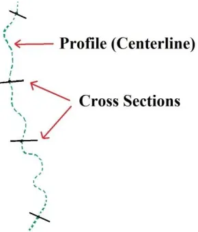
In particular for hydrographic surveying, these machines are used to calculate profiles and

cross-sections of certain areas. A profile is the centerline of a body of water. Cross-cross-sections are lines

Figure 2.1 A graphical representation of a profile (shown as a dashed line) and its corresponding

center lines (shown as solid lines).

For depth, a fathometer measurement is taken along the cross-sections and GPS coordinates are

taken in reference to a known benchmark. The depth is then subtracted from a vertical

benchmark to retrieve the elevation at the bottom of the channel. Once this survey data is

gathered, it can be used to interpolate the elevation for the given area and ultimately create

Digital Elevation Models (DEMs). These traditional survey techniques are proven to be very

precise [3].

Despite this precision, there are still short comings to these methods and they are phasing out in

favor of remote surveying methods. For example, when centerlines are unable to be gathered

from a survey,the centerline can easily be obtained from aerial photography or other data

sources. Surveying is an expensive and laborious process due to its hands on physical nature and

the need for expensive machinery. Remote methods can provide dense information without the

Light Detection and Ranging (LiDAR) has been a widely used survey method for the creation of

Digital Elevation Models (DEMs) [4]. The remote sensing method LiDAR uses pulsed laser light

to measure distances to the Earth [5]. Using this gathered distance information, as well as

information recorded by the aerial system, accurate and precise three-dimensional information is

generated about the surface below. LiDAR machinery is typically made up of a laser, a scanner,

and a GPS receiver, all mounted to a helicopter, airplane, or even an Unmanned Aerial Vehicle. The laser is beamed from the aircraft onto a targeted area on the Earth’s surface. This can be

anything from land or buildings, to bodies of water. The laser’s light is bounced off the object,

reflected, and recorded by a sensor which measures the distance, also known as range. The GPS

position and orientation are simultaneously recorded, and when combined with the range,

provide a set of elevation points for the area measured. Each point in the set comes complete

with latitude, longitude, and height for that particular spot of terrain, providing a set of detail-rich

information [5].

The use of different types of lasers in this process adds versatility to LiDAR methods. LiDAR

can be used topographically to survey land and any natural or manmade adaptations to it. For this

application, a near infrared laser is used for range measure. LiDAR can also be used

bathymetrically to survey the land under bodies of water and the variations in seafloor relief [6].

For this application, green laser light is used for range measure, due to its water-penetrating

abilities [5]. Unfortunately, LiDARs application for hydrographic surveying is problematic. Due

to the refractive properties of water, collected data can become distorted [7]. Also, sediment and

floating vegetation can block laser light from reaching the surface below, giving false results to

Figure 2.2: LiDAR Image – FEMA LiDAR Dataset Louisiana 2006 [15]

2.2 Digital Survey Data

Terrain data gathered through any of these types of surveying is digital and can be displayed with

three digital models: Digital Terrain Models (DTM), Digital Surface Models (DSM), or Digital

Elevation Models (DEM) [4]. The digital terrain data allow for a wide variety of applications

involving terrain, such as database management, hydraulic simulations, or even video games.

These three types of digital models have small fundamental differences. DSMs represent the

surface of the earth in its entirety with any and all manmade or natural objects present. DTMs

represent only the bare ground of a surface.

DEMs are used specifically for models that can be represented in a raster [8]. A raster is a type of

grid which contains coordinate information in Geographical Information Systems. In a LiDAR

location of that coordinate. Together the information in the raster makes a heightmap. These

heightmaps can be viewed as 8-bit grayscale images where the whitest values represent a higher

elevation and the blackest areas represent the lowest elevation [8]. Slope information for a pixel

can also be determined from DEMs. After determining the elevation of a particular pixel color,

the slope can be calculated between adjacent pixels through use of a matrix-like data structure

and slope formulas [9]. Having all of this information available from one model makes DEM

3 Model Development Algorithms

For cases pertaining to Louisiana waterways, several model development algorithms have been

studied. Of these popular algorithms, those which use raster data, such as Inverse Distance

Weighting functions, and those which utilize vector data, such as Delaunay triangulation and The

Hydraulic Spline algorithm, have been achieved. Although these methods all produce data, some

have proved to be more viable than others for various reasons. This section details these

techniques, their short comings, and methods for improvement in order to produce accurate and

precise surface models.

3.1 Current Modeling Techniques

Several techniques exist for transforming survey data into surface models. Delaunay

triangulation is one of the most commonly used methods [7]. Delaunay triangulation is

performed on survey data points, transforming them into a set of triangles which can be used as a

model. Delaunay Triangulation has its short comings for specific USACE applications. LiDAR

data taken for Louisiana waterways have not been able to reliably capture inundated terrain. To

compensate for these areas, cross-section surveying is done to obtain sparse, but accurate

elevation information on these waterways. The data are then merged with dense LiDAR to obtain

a complete model for an area. However, Delaunay Triangulation was found to be insufficient on

merged datasets with varying resolution. This can be seen in Figure 3.1. The sparse cross-section

data, seen in dark lines, are sparse compared to the LiDAR imagery seen in light grey.

Triangulation cannot be performed when there are not enough data points. In order for Delaunay

Figure 3.1: Merged surface point data [7].

Another method of creating surface models is through the Inverse Distance Weighting function

(IDW). IDW utilizes LiDAR and cross section raster data to produce a DEM. Functions are run

on coordinates with known elevation to predict areas of unknown elevation. However,

predictions are limited to coordinates that exist within a certain distance from the input data

points. This limits the functions ability to fill in holes and, much like Delaunay triangulation,

sparse cross section data results in a partially completed model [7]. To show this, IDW was

performed on the same data shown in Figure 3.1. It is presented in Figure 3.2. The data on which

it was performed contained insufficient cross section data for the entire water way to be

Figure 3.2: A surface raster generated using an inverse distance weighted function [7].

Flanagin1 proposes the Hydraulic Spline Algorithm, a generalization of the Waterway

Generation Algorithm, as a solution to this problem [7]. The Hydraulic Spline Algorithm uses

cross section data to generate hydraulic spline grids of any desired resolution. These grids can

then be merged with LiDAR to create a complete surface model for waterways. This algorithm

has been successfully executed on several USACE projects to prove its performance and

usefulness. While it does produce viable results, its method of grid generation is cumbersome.

The Hydraulic Spline Algorithm produces a vector surface which then must be manipulated

through Inverse Distance Weighting interpolation in order to generate a grid. If the hydraulic

spline were implemented with raster data instead of a vector surface, this interpolation would not

be necessary. The goal of this project is to perform a thorough analysis of the Hydraulic Spline

Algorithm and present the needed steps for a raster database implementation. In the following

1

section a detailed description of Flanagin’s Hydraulic Spline Algorithm is explained in order to

address the needs of a raster based interpretation.

3.2 The Hydraulic Spline Algorithm

The Hydraulic Spline Algorithm utilizes several techniques for data manipulation, such as

Hermite splines, cross section and profile intersections, Cartesian to spherical coordinate

conversion, profile supplementation, and polygon creation [7]. The algorithm is organized into

three components: 1) Hydraulic Spline Setup, 2) Supplementation of the centerline, and 3)

Polygon creation from spline evaluation.

Splines have long been used as an algorithmic tool in graphics for producing smooth curves and

surfaces [7]. In the Hydraulic Spline Algorithm, splines are used to produce a two-dimensional

irregular grid of quadrilaterals. It is these quadrilaterals that are used to reconstruct the

underwater terrain. A spline is defined by its control points which map a normalized position

along the curve. Most splines can be divided into two types, approximating and interpolating.

Approximating splines, such as Bezier and B-splines, use a set of control points to define the

shape of an output. Interpolating splines, such as Hermite splines, interpolate values throughout

the given control points. Interpolating splines also have the ability to preserve input vertices. It is

for this reason that they are chosen to be used in the Hydraulic Spline Algorithm. Specifically,

the Kochanek-Bartels spline, a type of Hermite spline, is used because it has the ability for the

user to define its control parameters for tension, bias, and continuity. The equation for this spline

Equation 1:

[ ]

In equation one and are standard Hermite spline control points. and are

additional control points which are used to define a consistent curvature. b represents the bias of

the curvature. The bias controls how far in front of or behind a control point the curvature is

allowed to reach. c represent a curvatures continuity, which determines how smooth the change

in slope is from one curve section to the next. t represents the tension. The value of these

parameters ranges between -1 and 1.

In order for the splines to produce a linked mesh of quadrilaterals it is important that the cross

sections are comprised of the same number of points [7]. The number of points also controls how

detailed the resulting grid will be. Having many points in a cross-section allowed many spline

quadrilaterals to be produced. The more quadrilaterals there are, the more detailed the grid. For

each point on a cross section a Kochaneck-Bartels spline is used for the x, y, and z components.

Because the output grid is two dimensional, two template splines are created. The tension

parameter of these template splines is copied to all of the other splines so that the user has control over the output of the cross section’s tension. A high tension, for example a value of 1,

will produce a straight line of splines. A lower tension, closer to -1, would produce curvy splines.

The centerline and cross sections are evaluated and their points of intersection are found. Only

cross sections that intersect the profile are used. If a cross section exists that does not lie on the

center line, it is not evaluated. The intersections are found by taking the Euclidean distance of the

the total length of the center line. This is shown in Figure 3.3. The distance is calculated in lines

one through five.

Algorithm 1

1 for i =1 to size(CrossSections) do

2 𝑃 ← 𝐶𝑟𝑜𝑠𝑠𝑆𝑒 𝑖𝑜𝑛𝑖 ∩ 𝑃𝑟𝑜𝑓𝑖𝑙𝑒;

3 𝑎𝑙 ℎ𝑎𝑠 𝑖 ← 𝑑𝑖𝑠 𝑎𝑛 𝑒 𝑓𝑟𝑜𝑚 𝑃𝑟𝑜𝑓𝑖𝑙𝑒 𝑒𝑛𝑑 𝑜𝑖𝑛 𝑜 𝑃 𝑙𝑒𝑛𝑔 ℎ 𝑜𝑓 𝑃𝑟𝑜𝑓𝑖𝑙𝑒 ;

4 end

5 for j = 0 to NumberOfCrossSectionSamples do

6 for k = 0 to size(CrossSections) do 7 𝑀 ← 𝑚𝑖𝑑 𝑜𝑖𝑛 𝐶𝑟𝑜𝑠𝑠𝑆𝑒 𝑖𝑜𝑛_𝑘 ;

8 Compute 𝑟, 𝜃, 𝜑 for 𝐶𝑟𝑜𝑠𝑠𝑆𝑒 𝑖𝑜𝑛_𝑘[𝑗] relative to M;

9 AddPoint(splines(j), alphas(k), 𝑟, 𝜃, 𝜑 );

10 end

11 end

Figure 3.3: Setting up the Hydraulic Spline Algorithm [7].

The remainder of Algorithm 1 (lines five through eleven) shows the setup of the splines for each

point. In Figure 3.4 the spline generation is shown. The red lines represent spline point

associations. Since each cross section has the same number of points, a distinct spline is created

for point position. The first points in all cross sections correspond to the first spline. The second

points in all cross sections compose the second spline. This is true for every point in every cross

Figure 3.4: Spline set up [7].

Also calculated in Algorithm 1 is a computation to change the coordinate system. This is done to

prevent problems caused by the natural bending of waterways. The Cartesian coordinates for the

splines are converted to spherical coordinates using Equation 2.

Equation 2:

𝑟 √

𝜃 ( )

The midpoint of the cross section is used as the logical origin for this conversion and the

coordinates at each cross section point are converted.

To produce viable results, it was determined that the profile should be supplemented. Cross

sections can be spaced overly far apart in some data [7]. When this is the case spline

interpolation can cause problems, such as aliasing, which is when different signals become

indistinguishable from one another during sampling. Flanagin shows that this is a specific

problem for hydrographic surveying, showing that the deepest path of a channel, called the

thalweg, has the potential to disappear and reappear in different locations. To solve this Flanagin

proposes the addition of auxiliary profile lines, one on each bank of the water way, to control the

transitions between cross sections. The solution is fleshed out in Algorithm 2:

Algorithm 2

1 𝑅𝑒𝑠𝑎𝑚 𝑙𝑒𝑑𝐶𝑒𝑛 𝑒𝑟𝑙𝑖𝑛𝑒𝐴𝑙 ℎ𝑎𝑠 ← ∅;

2 𝐶𝑒𝑛 𝑒𝑟𝑙𝑖𝑛𝑒𝐴𝑙 ℎ𝑎𝑠 ← 0.0 ∪ 𝐶𝑒𝑛 𝑒𝑟𝑙𝑖𝑛𝑒𝐴𝑙 ℎ𝑎𝑠;

3 𝐶𝑒𝑛 𝑒𝑟𝑙𝑖𝑛𝑒𝐴𝑙 ℎ𝑎𝑠 ← 𝐶𝑒𝑛 𝑒𝑟𝑙𝑖𝑛𝑒𝐴𝑙 ℎ𝑎𝑠 ∪ {1.0};

4 𝑃𝑜𝑖𝑛 𝑠𝑃𝑒𝑟𝐵𝑖𝑛 ← 𝑁𝑢𝑚 𝑒𝑟𝑂𝑓𝐶𝑟𝑜𝑠𝑠𝑆𝑒 𝑖𝑜𝑛𝑆𝑎𝑚 𝑙𝑒𝑠 size 𝐶𝑒𝑛 𝑒𝑟𝑙𝑖𝑛𝑒𝐴𝑙 ℎ𝑎𝑠 ;

5 fori = 1 to size(CenterlineAlphas) - 1 do 6 forj = 1 to size(PointsPerBin) -1 do

7 𝑅𝑒𝑠𝑎𝑚 𝑙𝑒𝑑𝐴𝑙 ℎ𝑎𝑠 ← 𝐶𝑒𝑛 𝑒𝑟𝑙𝑖𝑛𝑒𝐴𝑙 ℎ𝑎𝑠_𝑖+ 𝑗 1 𝐶𝑒𝑛 𝑒𝑟𝑙𝑖𝑛𝑒𝐴𝑙 ℎ𝑎𝑠_{𝑃𝑜𝑖𝑛 𝑠𝑃𝑒𝑟𝐵𝑖𝑛} 𝑖+1 ;

8 end

9 end

The left and right bank lines are used as additional centerlines. The normalized distance is found

for cross sections and auxiliary profile intersections. Ranges are created for the cross section

lines between the center profile and each bank line profile. First the alpha values are found for

the left and right endpoints of a cross-section line. The values are then split with the alpha value

of centerline intersection. The cross section points, the number of which is denoted as

PointsPerBin, are evenly distributed among the ranges such that each range has the same number

of points. For example, if the number of cross section points is forty, there will be ten points on

the left descending bank, then points on the left side of the channel, ten points on the right side of

the channel, and ten points on the right descending bank. This alters the way the grid would

otherwise be produced. Without this part of the algorithm points would be evenly distributed

along the centerline, as would the resulting polygons for that area. Now the points will be

distributed such that the concentration relies on the length of the range. If a range is shorter than

another, a greater concentration of polygons will result in that area. This results in more detail for

certain areas, such as the thalweg.

Now that the splines have been properly constructed, they are ready to be evaluated so that the

Algorithm 3

1 fori = 1 to NumberOfProfileSamples - 1 do

2 forj = 1 to NumberOfCrossSectionSamples -1 do

3 CreatePolygon 𝑃_{𝑖 1}𝑗 1, 𝑃_{𝑖 1}𝑗 , 𝑃_𝑖𝑗, 𝑃_𝑖𝑗 1 ;

4 end

5 end

Figure 3.6: Evaluating splines for the creation of polygons [7].

Algorithm 3 evaluates splines at regular intervals along the centerline and output cross sections

are produced. The NumberofProfileSamples and NumberOfCrossSectionSamples are defined by

the user. Flanagin presents a graphical representation of this method as well [7]. It can be seen in

Figure 3.7. Here, there are M number of profile samples which corresponds to the number of

cross sections in the data. There are also N number of cross section samples, which correspond to

the number of data points on a cross section. These follow the original profile of the waterway,

and the shapes are determined by the original cross sections of the waterway. In Figure 3.7 the

dashed green lines represent the created mesh. The solid green line represents the current mesh

polygon that is being created. The red line represents the profile centerline, with capital letters

Figure 3.7: A graphical representation of mesh generation [7].

Once an acceptable mesh is generated, it can then be merged with LiDAR data. However, this

data is exported in the form of vector output, which can be a problem. For many digital

applications raster data is preferred. In order for this vector data to be rasterized, a dense version

of the vector surface is exported and IDW interpolation is used to generate a raster. This adds a

step that makes the use of the Hydraulic Spline Algorithm more cumbersome. The process can

be streamlined by changing the output of the algorithm from a vector surface to a raster surface.

To do this the Hydraulic Spline Algorithm will need to be performed on a raster data set instead

of a vector data set. This would essentially develop a raster oriented process for the Hydraulic

Spline Algorithm. The next section details the advantages raster output would have over the

3.3 The Comparative Advantages of Raster Data in Geospatial Applications

Geospatial data can essentially be divided into vector and raster based information. Both have

practical applications and are necessary for the study of topology. However, vector data must

overcome several challenges when it comes to data storage [10]. This gives it a major

disadvantage of usefulness when compared to raster data, which is easier to store.

Vectors must use complex data structures in order to retain their information. Due to the

graphical nature of vectors, they can also be expensive to visualize. A significant amount of

specialized commercial software has been developed with the expressed intent of displaying and

manipulating geographical vector data. These products have been created out of necessity,

showing that vector data can be hard to work with. Additionally, these software products can be

expensive and require vast computing power. Raster data, on the other hand, is much simpler.

Gridded image data requires no complex data structures and can even be stored in geospatial

databases with ease [9]. The technology needed to display raster data is on par with viewing

most image data, and thus is accessible and inexpensive [10].

Vector data is often converted to raster data in order to manipulate it in ways that come more

naturally to raster data. Sometimes it is necessary to develop raster-oriented solutions for an

application that only possesses a vector-oriented solution [11]. Such is the case with the

Hydraulic Spline Algorithm, as a raster-oriented solution would remove unnecessary steps.

Another advantage of raster data is that it can relatively easily be converted to vector data [11].

This is good for vector data that has been converted to raster data for processing reasons.

complexity of the data and allows it to be better utilized. If the need arises for vector data, it can

simply be converted back.

It is actually possible to easily manipulate raster data in a database, giving it another edge over

vector data [9]. This has been proven to be computationally cheap, and also eliminates the need

for expensive vector processing software and machinery. Due to recent advances in geographic

database techniques, a raster based Hydraulic Spline algorithm could be implemented in a

database. This would make the Hydraulic Spline algorithm more practical by eliminating the

need to store vector data, and less laborious to implement by removing the need for specialized

software. The next section outlines a possible method for producing raster output with the

hydraulic spline algorithm.

3.4 A Raster Based Hydraulic Spline Approach

In order for the Hydraulic Spline Algorithm to be replicated as a raster based method, all of its

major components must be implementable on rasters. As described in section 3.2, this algorithm

is made up of three components: 1) Hydraulic Spline Setup, 2) Supplementation of the

centerline, and 3) Polygon creation from spline evaluation.

Following the Hydraulic Spline Algorithm 1, an initial set up of the spines is necessary. First the

cross section and profile line of the raster must be established. Due to the nature of raster grids,

each pixel also holds the geographic coordinate for that area. A search can be executed on all the

pixels of a raster to determine if the coordinates match up with those of the cross sections and

profile line. Finding the cross section and profile intersections is done by finding those pixels

which have coordinate values matching both centerline coordinates and cross section

solid line is a cross section, and the grid represents individual pixels. The pixel chosen through

search is outlined by a red box. This method also accomplishes the task of removing cross

sections that do not intersect the profile.

Figure 3.8: A representation of selecting profile cross section intersecting pixels in raster data.

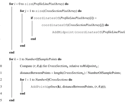
The pixels chosen at these midpoints become the local origin for interpolating sample points

along the cross section. By fetching the Cartesian coordinates from these sample points, they can

then be converted into spherical coordinates using the method mentioned in section 3.2. With the

new coordinates generated, splines are established at the corresponding locations, and the

necessary steps for Algorithm 1 are complete. A new Algorithm 1 is created to follow this

1 fori = 0 to size(ProfileLinePixelArray) do

2 forj = 1 to size(CrossSectionPixelArray) do

3 ifcoordinatesOf(ProfileLinePixelArray[i]) =

4 coordinatesOf(CrossSectionPixelArray[j]) do

5 AddMidpoint(coordinatesOf(ProfileLinePixelArray[i]);

6 end

7 end

8 end

9 fork = 1 to NumberOfSamplePointsdo

10 Compute (𝑟, 𝜃,ϕ) for 𝐶𝑟𝑜𝑠𝑠𝑆𝑒 𝑖𝑜𝑛𝑘 relative to𝑀𝑖𝑑 𝑜𝑖𝑛 𝑘;

11 distanceBetweenPoints = length(𝐶𝑟𝑜𝑠𝑠𝑆𝑒 𝑖𝑜𝑛_𝑘) / NumberOfSamplePoints;

12 forl = 1 to NumberOfCrossSectionsdo

13 AddPoint(splines(k), distanceBetweenPoints, (𝑟, 𝜃,ϕ));

14 end

15 end

Figure 3.9: Algorithm 1: Setting up splines in raster space

Following Algorithm 2, supplementary profile lines are added. They are established by searching

for the pixels which match coordinates for bank lines. Figure 3.10 shows where these profiles,

the long horizontal lines, would lie on sample LiDAR data. The short vertical lines represent

possible cross sections. Points can now be redistributed to evenly lie on the ranges generated.

Figure 3.10 shows raster data with highlighted pixels for cross sections, center profile, and

Figure 3.10: Supplementing the center line.

The Algorithm for this method of center line supplementation is as follows:

1 PointsPerBin = NumberOfSamplePoints / (NumberOfBanklines + 2);

2 fori = 1 to NumberOfBanklinesdo

3 forj = 0 to size(𝐵𝑎𝑛𝑘𝑙𝑖𝑛𝑒𝑃𝑖 𝑒𝑙𝐴𝑟𝑟𝑎 𝑖) do

4 fork = 0 to size(CrossSectionPixelArray) do

5 ifcoordinatesOf(BanklinePixelArray[j]) =

6 coordinatesOf(CrossSectionPixelArray[k]) do

7 AddBreakpoint(coordinatesOf(BanklinePixelArray[j]);

8 end

9 end

10 end

11 for n = 1 to NumberOfCrossSectionsdo

12 StartingPoint = FindNearestEndpoint(𝐵𝑟𝑒𝑎𝑘 𝑜𝑖𝑛 𝑛);

13 ResamplePoints(StartingPoint, 𝐵𝑟𝑒𝑎𝑘 𝑜𝑖𝑛 𝑛, PointsPerBin);

14 ResamplePoints(𝐵𝑟𝑒𝑎𝑘 𝑜𝑖𝑛 _𝑛, 𝑀𝑖𝑑 𝑜𝑖𝑛 _𝑛, PointsPerBin);

15 end

16 end

For Algorithm 3, the splines are evaluated to set the pixel values to their proper elevation. This is

done using Minimum Bounding Rectangles (MBR). The interpolated splines have created

polygons between the sampled points. MBRs can then be used to find all pixels between the

coordinates of these polygons. For each set of pixels found, the proper elevation is determined

and set within the raster. A diagram of this is shown in Figure 3.12. The MBR area is shown in

yellow. Red pixels represent spline control points. The green line is the profile of the waterway.

Algorithm 3 shown in Figure 3.12 shows the steps needed to create the polygons.

Figure 3.12: The bounding box area of raster pixels

1 fori = 1 for size(Midpoint) - 1 do

2 forj = 1 for size(crossSectionPoints) - 1 do

3 CreatePolygon(𝑃_𝑖𝑗, 𝑃_{𝑖 1}𝑗 1);

4 end

5 end

4 Implementation

This project is implemented in Oracle, which utilizes the features of Oracle Spatial and Graph

GeoRaster [14]. Oracle PL/SQL is used to define all data models as well as to manipulate the

data. Oracle 12c provides new functionality for manipulation and storage of raster data. Some

Extract, Transform, Load (ETL) Tools were also utilized, such as the Oracle GeoRaster Loader

and Oracle Spatial shapefile loader. The Geospatial Data Abstraction Library (GDAL) was used

to transform raster data into the format required of Oracle Spatial. Database diagrams were

created using Gliffy, a free online diagram utility.

4.1 Oracle Data Storage

GeoRaster is a built-in feature of Oracle Spatial and Graph. It allows the user to store, index,

query, analyze, and deliver raster image data, gridded data, and any associated metadata [13].

GeoRaster can be used not only to store DEMs but also DTMs and other gridded data [9].

GeoRaster data models are logically layered and multidimensional. Oracle Spatial has several

useful components for the management of raster data. MDSYS is the oracle schema. It defines

the storage, syntax, and semantics for both vector and raster geometric data types. Oracle Spatial

provides the SDO_Geometry data type for the storage of spatial data. It contains all the features

and capabilities of an oracle data. SDO_Geometry tables can be created and are fully functional

with database features such as views and triggers. Having a complete set of functionality is

essential for the manipulation, storage, retrieval, and relate-ability of raster data.

When GeoRaster database objects are created to represent an image, data has the ability to be

controlled on the pixel level. This is done by forming the data into a multidimensional array of

cells and pixels to be used interchangeably. The depth of a cell is stored as the data size of each

pixel. This defines a range for all the cell values and applies to each single cell.

Multidimensionality is expressed through layered banding of raster imagery. The number of

dimensions an array has is directly related to the type of imagery. Images that have RGB values

are usually stored as three dimensional arrays [9]. This allows each RGB value for a pixel to be

stored as its own byte value. In contrast, DEMs are usually portrayed in black and white so they

are stored in one dimensional arrays. In the case of DEMs, only one value is needed to represent

a pixel, and that is the elevation value. The dimensionality of the array also dictates the banding

of an image. Red, green, and blue images have three bands, while DEMs have one. Oracle

GeoRaster utilizes a generic data model in order to allow for many different types of pixels and

sizes [9]. Figure 4.1 represents the multidimensionality of the raster data model. The array on the

top shows a three dimensional array used to store red, green, and blue color values of a pixel.

Figure 4.1: Raster Data Models

GeoRaster data models get coordinate information from metadata, which can provide the proper

spatial reference system [13]. Spatial reference systems associated with a raster define the map

projection used to create Earth-based coordinates. Using this information the proper coordinates

are associated with each pixel in the raster array.

GeoRaster also supports the storage of pyramid levels. In Oracle, pyramids become a subobject

group of the GeoRaster Object [12]. These subobjects hold information pertaining to the degree

of resolution of raster data. Pyramid levels symbolize how much of the raster data has been reduced. As a pyramid level’s value increases, the resolution of the object decreases. Different

in an application. For this project, pyramid levels of zero are employed, signifying that the

largest resolutions available are utilized.

Oracle allows for a variety of methods for loading raster data into a geoRaster database [14].

Extract, Transform, Load (ETL) tools are particularly useful in this phase of implementation.

Oracle Spatial example files contain a complete set of ETL tools, based in java, for loading,

viewing, and exporting GeoRaster data. They are standalone executables designed to run in a

Java Virtual Machine. Since java is so closely integrated with Oracle database, this makes the

GeoRaster ETL tools convenient and easy to use.

4.2 Methodology

Spatial data requires a fully designed, specified model for the storage of data [9]. In this regard, it

is no different from other databases. A well designed spatial database is the first step to store

raster data. Figure 4.2 diagrams the needed tables for a GeoRaster database.

An Oracle GeoRaster database requires two tables to store a raster object. The first table, the

GeoRaster table, indexes and keeps track of the GeoRaster objects. The second table, the raster

data table, holds the key of the object, the tablespace that holds it, and other necessary

information for handling raster data. This information is required for the raster data table,

because it manages the storage of the actual data. The raster data table manages raster data as

Large Object (LOB) datatypes, which are colloquially referred to as blocks of data. LOBs are

Figure: 4.2 GeoRaster Database Diagram

In order to create the necessary data blocks, the multidimensional arrays of pixel values must be

linearized. The method for doing this is called band-sequential (BSQ) linearization [9]. In this

process, raster data is transformed into a linear sequence of bytes and stored. There are many

tools with the ability to perform BSQ linearization on raster data. Oracle recommends using the

Geospatial Data Abstraction Library (GDAL) [14]. The GDAL utility has a translate function,

gdal_translate, which reformats and reblocks the raster. Using the function creates a new

striped file that is based on the original raster data. Once that data has been translated, it is ready

to be stored in the database.

Before data can be loaded, the GeoRaster database design must be implemented. First, the

tablespace must be created. The tablespace defines the storage location where the actual raster

before instantiating tables so that the proper storage allocation can take place. A sample

tablespace declaration would be:

create tablespace USER_DATA

datafile 'C:\app\USER\oradata\GISDB\DATAFILE\01_user_data.dbf' size 1000m

extent management local autoallocate segment space management auto;

Next, two tables are created; one for the storage of the raster data, and one for the storage of

GeoRaster objects. The SQL for these tables is implemented below:

CREATE TABLE city_images (image_index NUMBER, image_description VARCHAR2(50), image SDO_GEORASTER);

CREATE TABLE city_images_rdt OF SDO_RASTER

(PRIMARY KEY (rasterID, pyramidLevel, bandBlockNumber,

rowBlockNumber, columnBlockNumber))

TABLESPACE USERS_DATA

LOB(rasterBlock) STORE AS SECUREFILE(CACHE);

The city_images table holds index numbers, text descriptions of each image, and the

SDO_GEORASTER data column. The city_images_rdt table is a Raster Data Table

(RDT). As mentioned earlier, this is the table where the actual raster data is stored. A primary

key is used to enforce B-tree indexing on the raster data table. This table also utilizes Oracle

SecureFiles and Large Object (LOB) datatypes to store data in the needed format [14]. Data

The datafile declared here becomes the location for the raster data storage. User created

datafiles should be stored in the Oracle database architecture under the DATAFILE folder. This

is not mandatory but it follows the convention for creating stable databases [13]. Commands are

also issued to give the database automatic control over space management.

There are several options for loading GeoRaster data into the newly created database, such as the

GeoRaster ETL tools included in the Oracle Spatial example files. Oracle can also handle SQL

based import commands for GeoRaster data. The needed SQL commands are detailed in this

section.

When loading data through SQL implementation, permissions must be granted to the user

creating the tables, as well as to the Oracle schema MDSYS. These commands, seen below,

allow the system to read data for imputing it into tables.

call dbms_java.grant_permission( 'USER',

'SYS:java.io.FilePermission', 'C:\...\rasterFile.tif', 'read' )

call dbms_java.grant_permission( 'MDSYS',

'SYS:java.io.FilePermission', 'C:\...\rasterFile.tif', 'read' )

After permissions have been granted for the specified files, commands for importing data may be

implemented in the following manner:

DECLARE

geor SDO_GEORASTER;

BEGIN

INSERT INTO city_images

values( 1, 'Raster_TIFF_1_description_and_other_information', sdo_geor.init('city_images_rdt') );

WHERE image_index = 1 FOR UPDATE;

sdo_geor.importFrom(geor, 'blocksize=(256,256)', 'TIFF', 'file', 'C:\...\rasterFile.tif');

UPDATE city_images SET image = geor where image_index = 1;

END;

This SQL code first declares an empty GeoRaster object. This creates a space for the external

image data to reside. Sample data is inserted here as a session variable. This data includes an

index, description text, and an initialization for the raster data table, city_images_rdt. Now

that data has been initialized in the table, a Tagged Image File Format (TIFF) raster file can be

imported. To execute this, the previously created row is updated and the sdo_geor data

column is populated using the session variable data. The updated values include the object type,

data block size, compression type, quality, and location of the desired TIFF file source. The

block size denotes the number of cells per block. In this instance, the blockSize is set to 256

for the row dimension, 256 for the column dimension and has a band output width of one. If this

file had red, green, and blue color values, the band output width would be three and would be

represented in the blocksize as follows: blocksize=(256,256,3).

The GeoRaster Viewer, provided by Oracle as part of the GeoRaster ETL tools, displays

GeoRaster objects, metadata, and raster imagery through a specialized graphical user interface

[14]. Successfully stored raster data can be viewed by invoking the proper Java programs. These

programs must first be installed as part of the Oracle Spatial demo files. The GeoRaster Viewer

can also be used to validate metadata for the functions presented in this section. Figure 4.3 shows

Figure 4.3: The GeoRaster Viewer

Reading cell data out of the database is an exercise of this project. The process for doing so

includes a limited number of steps which are outlined in this section. As stated earlier in this

section, raster data is stored in the database as LOB data blocks. If the LOB data blocks are

stored as BLOBs, it will be necessary to convert this binary data from its raw state back into

standard SQL data types [9]. The following SQL creates a function called getValue.

CREATE OR REPLACE Function getValue(cellDepth Number, buffer1 raw, index1 Number, numType Number)

RETURN Number IS

R1 raw(1);

R2 raw(2);

R4 raw(4);

R8 raw(8);

BEGIN

IF cellDepth = 1 THEN

R1 := UTL_RAW.SUBSTR(buffer1, (index1-1) * cellDepth+1, cellDepth);

val := UTL_RAW.CAST_TO_BINARY_INTEGER(R1);

ElsIf cellDepth = 2 Then

R2 := UTL_RAW.SUBSTR(buffer1, (index1-1) * cellDepth+1, cellDepth);

val := UTL_RAW.CAST_TO_BINARY_INTEGER(R2);

ElsIf cellDepth = 4 Then

R4 := UTL_RAW.SUBSTR(buffer1, (index1-1) * cellDepth+1, cellDepth);

If numType = 0 Then

val := UTL_RAW.CAST_TO_BINARY_INTEGER(R4);

Else

val := UTL_RAW.CAST_TO_BINARY_FLOAT(R4);

End If;

ElsIf cellDepth = 8 Then

R8 := UTL_RAW.SUBSTR(buffer1, (index1-1)*cellDepth+1, cellDepth);

val := UTL_RAW.CAST_TO_BINARY_DOUBLE(R8);

End If;

Return val;

End;

getValue takes in a cell depth and a buffer of raw data. The cell depth is used to determine

what type of data is stored in the BLOB in order to output the data in the proper data type. Cell

UTL_RAW package is provided by SQL for manipulating raw data types [12]. The numType

parameter is used to denote if a value should be of type floating point or integer.

Now that it is possible to retrieve readable data from the database, manipulation techniques can

be explored. GeoRaster functionality includes several powerful tools for creating, modifying, and

retrieving information pertaining to GeoRaster objects [14]. The MDSYS.SDO_GEOR package in

particular contains many functions and procedures needed to create a raster interpretation of the

Hydraulic Spline Algorithm. One such feature utilized is the SDO_GEOR.getRasterSubset

function. This function creates a single LOB object containing all pixels, of a specified pyramid

level, that are inside or on the boundary of a specified rectangular window or polygon geometry

object (Oracle GeoRaster Doc). SDO_GEOR.getRasterSubset uses the minimum bounding

rectangle of the window or geometry object to find and return the requested pixels. Because of

the minimum bounding rectangle feature of this function, it can be used to retrieve and set pixel

values for spline evaluation. The function below uses SDO_GEOR.getRasterSubset to

return the average pixel value for an area within the minimum bounding rectangle.

An sdo_Number_array is sent in with the coordinates of the upper and lower pixels of the

bounding box. The SDO_GEOMETRY value is left null, denoting that the area of interest will be

calculated from data in cell space, not vector space. If vector space was desired, the

sdo_Number_array would be replaced with null and the SDO_GEOMETRY value would

instead be filled.

CREATE OR REPLACE FUNCTION getAvgCellValue

cellWindow sdo_Number_array, geomWindow SDO_GEOMETRY)

Return Number As

cellType Varchar2(80);

numType Number := 0;

cellDepth Number; parm Varchar(200); lb blob; buffer1 raw(32767); tempAmount Integer; amount Integer; offset Integer; length Integer; value Number; BEGIN cellType := geoRastObj.metadata.extract('/georasterMetadata/rasterInfo/ cellDepth/text()', 'xmlns=http://xmlns.oracle.com/spatial/georaster').getStringVal( );

IF cellType = '32BIT_REAL' Then

numType := 1;

END IF;

cellDepth := SDO_GEOR.getCellDepth(geoRastObj);

IF cellDepth < 8 Then

cellDepth := 8;

parm := 'celldepth=8bit_u';

END IF;

dbms_lob.createTemporary(lb, true);

IF (geomWindow Is null) Then

SDO_GEOR.getRasterSubset(geoRastObj,plevel,cellWindow,to_ch ar(bandNum),lb,parm);

ELSEIF (cellWindow Is null) Then

SDO_GEOR.getRasterSubset(geoRastObj,plevel,geomWindow,to_ch ar(bandNum),lb,parm);

END IF;

length := dbms_lob.getlength(lb);

cellDepth := cellDepth / 8;

amount := floor(32767 / cellDepth) * cellDepth;

tempAmount := amount;

offset := 1;

WHILE offset <= length LOOP

dbms_lob.read(lb, amount, offset, buffer1);

FOR i In 1..amount/cellDepth LOOP

value := value + (getValue(cellDepth, buffer1, i, numType));

END LOOP;

value := AVG(value)

offset := offset+amount;

amount := tempAmount;

END LOOP;

dbms_lob.freeTemporary(lb);

Return value;

END;

The getAvgCellValue function takes in a georaster object, pyramid level, band number, and

in both raster space and vector space [14]. For this reason the function takes in windows of both

types. Values are then instantiated for fetching cell data, calculating its average, and returning

the value. The buffer is set to the maximum amount of bytes readable for the raw data type,

32767 bytes. The metadata is called, from which the cell type is extracted, and proper cell depth

is determined. The function then creates a temporary LOB object to store the read data for

calculation. The type of window used, cell based or vector based, is determined and the

SDO_GEOR.getRasterSubset function is called for those values. The values in the LOB

object are read and averaged. The temporary memory in the LOB is released and the average is

returned. getAvgCellValue can be called in the following manner:

SELECT getAvgCellValue(raster, 0, 0, sdo_Number_array(0,0,551551), null)

FROM city_images WHERE id=1;

One advantageous feature of Oracle Spatial is its ability to convert raster cells to model types in

vector space [13]. This is utilized in problems where the raster based data does not provide

sufficient information. Additionally, combining raster and vector analysis functions in PL/SQL

preserves the efficient nature of database manipulation, as it requires no external vector

processing software or equipment. Some model types needed for creating a raster based

hydraulic spline method are points and polygons. This section details the functions needed to

create points and polygons for raster data.

In order for raster space to be converted to vector space, the corresponding objects must exist in

the same coordinate space. Additionally, resolution of the raster must be known so that a proper

one-to-one coordinate mapping method can be established because resolution tells how much

can be found in the metadata. It should be verified before implementing any cell to model space

conversion. Another key difference in vector and raster space is the origin for coordinate

mapping. In vector space coordinates are mapped with a lower-left corner origin, while in raster

space coordinates are mapped with an upper-left corner origin. To adjust this, models may need

to be flipped in some functions in order for a proper mapping to be produced [9]. The first step of

converting cell coordinates to point geometry is to fetch the coordinate values of the raster.

Oracle provides this functionality, which can be seen in the example below.

SELECT sdo_geo.getCellCoordiante(georaster, 0,

SDO_GEOMETRY(2001,82394,sdo_point_type(3234.64,7489527.23,n ull,null)) coord

FROM city_images WHERE georid = 1;

The coordinates are returned as a SDO_NUMBER_ARRAY. This array can be used to send

coordinate information to a function which will create a geometry in cell space. Such a function

will be called cellGeometry and is outlined below.

CREATE OR REPLACE FUNCTION cellGeometry (rowCoord number, columnCoord number, georaster sdo_georaster, geomType number)

Return SDO_GEOMETRY Is

mbr SDO_GEOMETRY;

spatialResolution sdo_number_array;

xResolution Number;

yResolution Number;

xOffset Number;

yOffset Number;

Begin

spatialResolution :=

sdo_geor.getSpatialResolutions(georaster);

xResolution := spatialResolution(1);

yResolution := spatialResolution(2);

xOffset := mbr.sdo_ordinates(1) + columnCoor*xResolution;

yOffset := mbr.sdo_ordinates(4) - rowCoord*yResolution;

IF (geomType Is NULL) THEN

geomType = 2001;

END IF

Return SDO_GEOMETRY(geomType, mbr.sdo_srid, null, sdo_elem_info_array(1, 1003, 3),

sdo_ordinate_array(xOffset, yOffset – yResolution, xOffset+xResolution, yOffset));

End;

Coordinates of a cell and the host raster are taken into the cellGeometry function. Variables

for the geometry calculation, resolution, and offset are created and instantiated using SDO_GEOR

functionality. Then, the y values are flipped to accommodate the change in coordinate origin

mentioned earlier. The new geometry is instantiated as a point type, denoted by the number

2001, and is returned.

The points of the minimum bounding rectangle are derived from the SDO_ORDINATE_ARRAY.

In this array, maximum and minimum values for x and y points are stored such that

SDO_ORDINATE_ARRAY(xMinimum, yMinimum, xMaximum, yMinimum).These

values are fetched from the minimum bounding rectangle by calling

mbr.sdo_ordinates(arrayIndex). In the cellGeometry function the minimum

x and y. This gives the information needed to determine the points where the SDO_GEOMETRY

will be created.

The cellGeometry function can be used as is for generating point models from raster data. If

geomType is specified as 2003 a polygon will be created. If geomType is specified as 2002 a

line will be created. Figure 4.4 illustrates the differences in these geometry types when applied to

raster data. Oracle’s method of creating geometric objects from raster data works by instantiating

SDO_GEOMETRY objects relative to provided coordinates. For a point, an object is set to

encompass only the specified point’s coordinates. For a line object, points are created with

straight arc segments and stored in a line string. For Polygons, the perimeter is made up of lines,

and all points encompassed by it are stored.

Figure 4.4: Raster to Vector Space Illustration

For creating polygon models, a minimum bounding rectangle for two points can be used. The

following function sends in raster data, pyramid level, and a set of minimum bounding rectangle

coordinates in the form of a SDO_GEOMETRY. All values of the SDO_ORDINATE_ARRAY are

Create Or Replace Function createPolygon( georaster sdo_georaster, plevel number, geomWindow SDO_GEOMETRY)

Return SDO_GEOMETRY Is

cellGeom SDO_GEOMETRY; colNum Number; rowNum Number; mbr SDO_GEOMETRY; minimumCorner sdo_number_array; maximumCorner sdo_number_array; xMin Number; xMax Number; yMin Number; yMax Number; Begin

mbr := sdo_geom.sdo_mbr(geomWindow);

xMin := mbr.sdo_ordinates(1);

yMin := mbr.sdo_ordinates(2);

xMax := mbr.sdo_ordinates(3);

yMax := mbr.sdo_ordinates(4);

minimumCorner := sdo_geor.getCellCoordinate(georaster, 0, SDO_GEOMETRY(2001,

mbr.sdo_srid, sdo_point_type(xMin,yMax,null),null,null));

maximumCorner := sdo_geor.getCellCoordinate(georaster, 0, SDO_GEOMETRY(2001,

mbr.sdo_srid, sdo_point_type(xMax,yMin,null),null,null));

For rowNum in minimumCorner(1) .. maximumCorner(1) Loop

For colNum in minimumCorner(2) .. maximumCorner(2) Loop

End Loop;

End Loop;

Return cellGeom;

End;

Points will need to be converted from Cartesian coordinates to spherical coordinates for correct

placement of splines [7]. Created geometries can be converted to different coordinate systems

using the SDO_CS.TRANSFORM function of Oracle Spatial [13]. This function can be

associated with different use cases and use plans for converting to different types. One use case

called USE_SPHERICAL performs the transformation in spherical math, allowing a geometry to

be transformed to spherical points. SDO_CS.TRANSFORM can be called as follows:

SDO_CS.TRANSFORM( SDO_GEOMETRY, USE_SPHERICAL, SDO_SRID);

A sdo_geometry with new coordinates is returned.

Oracle currently supports three main types of curves, Bezier curve, B-spline curve and NURBS

curve. With the release of Oracle Database 12c (12.1) support for Non-Uniform Rational

B-spline (NURBS) curve geometries was introduced [13]. NURBS curves represent curves through

control points and knots and can be used to represent cubic splines with little data. They require

three or more control points and allow the user to specify the exact amount. This allows for

splines with more than two control points, which is necessary to define a consistent curvature.

A NURBS curve is created as a SDO_GEOMETRY in the following manner:

SDO_GEOMETRY(

SDO_SRID,

SDO_POINT,

SDO_ELEM_INFO_ARRAY(offset, 2, 3),

SDO_ORDINATE_ARRAY

(3,

7,

x1, y1, w1,

x2, y2, w2,

x3, y3, w3,

x4, y4, w4,

x5, y5, w5,

x6, y6, w6,

x7, y7, w7,

11,

0, 0, 0, 0, 0.25, 0.5, 0.75, 1.0, 1.0, 1.0, 1.0))

The SDO_GTYPE for a NURBS curve should be set to the value ‘2002’ indicating it to be two

dimensional and a single line string. The SDO_ELEM_INFO_ARRAY holds the offset, element

type, and interpretation value. This array holds information for one element of type

SDO_ETYPE_CURVE with an interpretation value of three for NURBS curves. The

SDO_ORDINATE_ARRAY holds the degree of the NURBS curve, the number of weighted

control points, the locations and weights of these control points, the number of knot values, and

the normalized knot vector. For this example, the curve has a degree of three and seven control

points. The location of these points is denoted by their x and y coordinates (x1, y1 through x7,

y7) for each point and the weight of each point (w1 through w7). The number of knot values is

the sum of the number of control points and the degree plus one. The normalized knot vector is

equal to the degree of the curve plus one. Therefore, for this example there are four zeroes and

ones in the normalized knot vector, and values in between are evenly distributed until eleven

values exist. This approximates values across the spline.

4.3 Challenges

Splines are a major component and somewhat of a challenge for this project. The

Kochanek-Bartels splines used in the Hydraulic Spline algorithm are interpolating splines while NURBS

curves create approximating splines. Because Kochanek-Bartels splines and NURBS curves are

fundamentally different, this could cause issues with producing desirable results. However, some

properties of raster data can be utilized to counteract this drawback. Kochanek-Bartels splines

provide methods to manage spline curvature without calculating slope derivatives. Fortunately,

slopes can fairly easily be calculated with raster data, so it would not be computationally

expensive to do this.

Slope can be calculated from the pixel values of DEMs through several methods. One simple

method is to take the eight neighbors of a pixel into a matrix and calculate the rise over run [9].

For example, slope of a pixel, e, can be found by constructing the following matrix of elevation

values for e and its surrounding pixels:

𝑎 𝑑 𝑒 𝑓 𝑔 ℎ 𝑖

Now the following calculations can be determined:

𝑑 𝑑

𝑑 𝑑

𝑔 ℎ 𝑖 𝑎 ] [ 𝑅𝑒𝑠𝑜𝑙𝑢 𝑖𝑜𝑛]

𝑠𝑙𝑜 𝑒 𝑟𝑖𝑠𝑒

𝑟𝑢𝑛 √ 𝑑 𝑑 𝑑 𝑑

Pixel values can be retrieved and manipulated through the methods mentioned in the previous

section. Since DEMs can be very large precautions should be taken when performing these

calculations so that it remains quick and efficient. Small subsets of the raster should be retrieved

and processed rather than attempting to calculate the entire raster at once.

Implementing this project in an Oracle database has several advantages, but significant learning

curve is also present. Not only is a vast working knowledge of Oracle Spatial and Oracle

GeoRaster required, but the intricacies of managing large complex databases are also needed.

This can make database implementations out of reach for many individuals working with surface

models. A Java or C++ implementation would not require this knowledge and may be favored

for this reason. However, the advantages provided by direct manipulation of data through

PL/SQL far outweigh the ease of use provided by other technologies. Companies and

organizations with dedicated database management could more easily take advantage of an

5 Conclusion

The raster based method of spline creation provides more efficient data manipulation due to the

inherent properties of raster data. This project provides a well described method that can be

readily applied to topics mentioned in this chapter. Additionally, future work can still be done

within this field and is detailed below.

5.1 Possible Applications

Thematic raster data can be created from multi-spectral images [9]. Land cover data is an

example of thematic raster data that has discrete sets of values assigned to different pixels in the

raster. Here, numbers are stored which denote the type of land covered by a pixel space. Figure

5.1 shows the different types of land cover, the number of their classification, and the color of

the pixel for that type.

Due to the size of raster data, it could be advantageous to only select pixels based on their land

cover classification. This would reduce the cost of searching for or sorting pixels by only

focusing on a subset of the raster instead of every pixel value in the raster. This type of raster

would be beneficial for hydrographic surveying problems. Land Cover Classification would

allow an analyzer to select only Open Water data for analysis and manipulation. Since the data

are obtained as a subset of the raster, the functions presented in the previous sections would be

Figure 5.1: Land Cover Classification Chart [9].

5.2 Future Work

This raster based spline creation method has been interpreted for individual waterway channels.

In reality, hydraulic modeling projects encompass large networks of waterways, which contain

many branches, confluences, and forks [7]. The Hydraulic Spline Algorithm has been

successfully modified to account for these geographic occurrences. Further research would need

to be done to determine if confluences and waterway branching could be accommodated in a

raster based interpretation.

Possible issues could arise with the database implementation of NURBS splines presented in this

possible that NURBS splines may only be used for tight tension points such as channels. In the

future, NURBS should be tested on curvy waterways to see how the tension reacts in different

situations. If NURBS prove to be unusable in common waterway conditions there would be

sufficient need for database support of Kochanek-Bartels splines.

5.3 Summary

This project successfully outlines the method of improving surface model data by generating

splines in raster space. Working with raster data is shown to have many advantages over methods

utilizing vector data, including the Hydraulic Spline algorithm. Improving surface model data

and their subsequent creation methods is necessary for the advancement of work done by the U.