Adjusted permutation method for multiple attribute decision making with meta-heuristic solution approaches Pages 369-384 Download PDF

* Corresponding author. Tel.: +0989112713453 E-mail addresses: , Email:[email protected] (H. Karimi) © 2011 Growing Science Ltd. All rights reserved. doi: 10.5267/j.ijiec.2010.07.002

Contents lists available atGrowingScience

International Journal of Industrial Engineering Computations

homepage: www.GrowingScience.com/ijiec

Adjusted permutation method for multiple attribute decision making with meta-heuristic solution approaches

Hossein Karimia, Alireza Rezaeiniab

a

Department of Industrial Engineering, Shahed University, Tehran, Iran

b

Department of Industrial Engineering, Tehran University of Teacher Training, Tehran, Iran A R T I C L E I N F O A B S T R A C T

Article history: Received 1 July 2010 Received in revised form 13 October 2010 Accepted 14 October 2010 Available online 14 October 2010

  The permutation method of multiple attribute decision making has two significant deficiencies: high computational time and wrong priority output in some problem instances. In this paper, a novel permutation method called adjusted permutation method (APM) is proposed to compensate deficiencies of conventional permutation method. We propose Tabu search (TS) and particle swarm optimization (PSO) to find suitable solutions at a reasonable computational time for large problem instances. The proposed method is examined using some numerical examples to evaluate the performance of the proposed method. The preliminary results show that both approaches provide competent solutions in relatively reasonable amounts of time while TS performs better to solve APM.

© 2011 Growing Science Ltd.  All rights reserved.

Keywords: MADM

Adjusted permutation Tabu search

Particle swarm optimization

1. Introduction

There are many human-made decisions which are influenced by various conflicting factors. Organizations are typical examples of environments where different segments (departments) are in consistent conflict in terms of organizational objectives. In such a conflicting environment, multiple criteria decision making (MCDM) techniques are basically developed to select or rank decision alternatives. The existing conflict among goals of a decision maker implies that full attainment to a particular goal may jeopardize reaching the other objectives. In the past, business and industry decisions were used to have merely two determinants: the “boss”, and the resulting profit. Today, however, decision making may involve many people with multiple and conflicting criteria. To cope with this complexity, researchers are consistently looking for more capable MCDM techniques which could better capture the real situation of a decision making process.

focuses on problems with discrete decision spaces (Yoon & Hwang, 1981). MADM methods are classified into the following groups: 1) Compensatory methods where a production with high expenditure but good quality is compensated because of its high quality (Yoon & Hwang, 1981). ELECTRE, MDS, MRS, TOPSIS, SAW, Linear assignment are examples of this method. 2) Non compensatory methods where the attributes are separated. For instance, for taking driving license non compensative important factors such as normal eye test, driving rule test and practical driving examination are used where one’s strength in one of the tests does not compensate the others. Dominance, Lexicography, Elimination, Permutation are examples of this kind of model (Korhonen et al., 1992).

Each MADM methodology has its own limitations and attributes, and the decision maker cannot use one model for all decision-making problems. Using MADM methodology to prioritize various alternatives of a decision problem requires considering both the characteristics of the preferred methodology and the attributes of the problem itself. Nevertheless, there is always a chance of reaching to wrong priorities of the alternatives. The technique for order preference by similarity to ideal solution (TOPSIS) is a classical method to solve multi-criteria decision-making problem which was first developed by Hwang and Yoon (1981) and subsequently discussed by many such as Chu (2002), Olson (2004) and Peng (2000). According to TOPSIS, alternatives are chosen based on the shortest distance from the positive ideal solution (PIS) and the farthest distance from the negative ideal solution (NIS). The PIS has the best measures over all attributes, while the NIS has the worst measures over all attributes. TOPSIS was originally presented in the context of multiple criteria decision making, where the relative importance decision maker preference was a factor and subjective weights were inputs.

The analytical hierarchy process (AHP) method, as another MADM method, developed by Saaty (1990), is based on three principles: decomposition, comparative judgment and synthesis of priorities. Based on the decomposition principle, the decision problem is decomposed into a hierarchy that captures the necessary elements of the problem. The ELECTRE I method, originally introduced by Roy (1968), was built for multi-criteria choice problem where the primary aim is to obtain ranking for various alternatives. ELECTRE II was developed by Roy and Bertier (1971) where it represented an improvement on ELECTRE I. Just a few years later, ELECTRE III for ranking actions was devised by Roy (1978). Another ELECTRE method, known as ELECTRE IV, was introduced by Hugonnard and Roy (1982) as a technique for ranking the alternatives in a real-world project. The new method was equipped with an inserted outranking relationships framework. ELECTRE III is used when it is possible and desirable to express the quantity of the relative importance of criteria and ELECTRE IV is applied when this quantification is not possible.

Permutation method (PM) is one of the MADM techniques to find the best linear ordering of the alternatives. It is often difficult to reach the final result by PM since the method needs to spend tremendous amount of CPU-time which increases exponentially as the number of the alternatives increases. Also, Rinnooy (1976) proved that if the number of alternatives increases, the problem becomes NP-hard. Among all MADM approaches, permutation method is a technique developed to rank decision alternatives based on decision matrix and weights of criteria. This method is applied on a variety of industrial problems including location and allocation of factories in national or international level, establishment of efficient production and non-production units in factory environment, suitable layout design for equipment and machinery production units, selection of suppliers, etc. There are different goals and criteria which could be considered in the decision-making process such as working conditions, production requirements, practical constraints, and personnel requirements.

(1994) applied the method for analysis of recorded electrical wave datasets of brain. Chin and Haughton (1996) proposed permutation test for analyzing the student learning evaluations. Permutation methods were also applied by Pantazis et al. (2003) for the analysis of MEG data in reconstructed cortical maps of brain activation. Turskis (2008) used this method for contractor's evaluation. Chen and Wang (2009) presented interval-valued fuzzy permutation (IVFP) methods for solving MADM problems based on interval-valued fuzzy sets and showed how this method could be used in group decision makings. For more reviewing MCDM literature, interested readers can study Figueira et al. (2005).

In this paper, an adjusted permutation method (APM) is proposed to correct shortcomings of the classical permutation method. Since APM has the same complexity degree as the classical permutation method, tabu search (TS) and particle swarm optimization (PSO) techniques are proposed to handle large instances of the problem.

The remainder of this paper is organized as follows. Section 2 is dedicated to an introduction to the classical permutation method. The APM is proposed in Section 3. Two meta-heuristic techniques including TS and PSO are described in Section 4 to handle APM for large instances of the problem. Numerical examples are presented in Section 5. Finally, the paper is concluded in Section 6.

2. Classical permutation method

The permutation method for MADM problem was first proposed by Jacquet-Lagreze (1969). It is

based on the permutation of decision alternatives: If m alternatives are available, thenm!

permutations can be generated. This method calculates a rate for each permutation and eventually

chooses the permutation with the highest rate as the preferable permutation. Suppose there are m

alternatives(A₁,A₂,...,A_m) and the problem has n criteria (X1, X2, …, Xn).Then the decision matrix (D) can be formed with alternatives and criteria in rows and columns, respectively. In general, the importance of each criterion is different.

For instance suppose that there are three alternatives(m=3)which are displayed with A1, A2 and A3.

In this case, there are 3! =6 permutations as P₁={A₁,A₂,A₃},P₂ ={A₁,A₃,A₂}, P₃={A₂,A₁,A₃},

} , ,

{ _{2 3 1}

4 A A A

P = ,P₅ ={A₃,A₁,A₂}, and P₆ ={A₃,A₂,A₁}.

In order to choose the best permutation, we first define the concordance (C_kl)and the discordance

)

(Dkl sets. These sets are generated based on pairwise comparison of alternatives k andl regarding

the criteria. akj is defined as the performance of kth alternative in jth criterion in the decision

matrix. Suppose criterion j has positive effect on our decision. Now ifakj≥alj, Then j will be inCkl

set, otherwise j will be inDkl set. Mathematically speaking, the concordance and discordance sets

are defined as:

l k m l

k a a j

C_kl ={ | _kj ≥ _lj} , =1,2,..., ≠ ₍₁₎

l k m l

k a a j

D_kl ={ | _kj ≤ _lj} , =1,2,..., ≠ (2)

After generating C_kl and D_lk for a permutation, the rate of that permutation is calculated as follows,

! ,..., 1

, i m

w w

R

kl D j j kl

C j j

where R_i and w_j denote the rate of permutation P_i and the weight of criterion j , respectively. After

calculating these rates for all permutations, the permutation with the highest rate is selected as the best priority sequence of decision alternatives.

In the pairwise comparison of alternatives, the classical permutation method can only consider the priority of an alternative over the other one, and not the degree by which this priority exists. This shortcoming can be addressed through the following example. Suppose there are three alternatives and three criteria in a decision matrix given by Table 1.

Table 1

A sample decision matrix

Criterion

Alternative 1 (-) 2 (+) 3 (+)

1 200 5 2400

2 300 5 2420

3 350 3 2000

The first criterion has a negative effect and the other two criteria have positive effects on the decision. The weights of criteria are given as 0.3, 0.4, and 0.3, respectively. Assuming a linear utility function, it is clear that the alternative 1 is better than alternative 2. The classical permutation method, however, cannot underscore this dominance. It calculates the same rate of 2 for permutations

} , ,

{A₁ A₂ A₃ and {A₂,A₁,A₃} whereas the former is clearly the best permutation of this problem. To

address this drawback, the APM is proposed in the next section.

3. Adjusted Permutation Method

In APM, the rate of each permutation is calculated as follows,

! ..., , 1 , ) | | ( ) | |

( _{max min max min} i m

a a a a w a a a a w R kl C

j j Dkl _{j j}

lj kj j j j lj kj j

i ₋ =

− − − − = ′

_∑

_∑

∈ ∈ (4)

where amax_j and amin_j are the maximum and the minimum values of the jth criterion, respectively. The

first and the second terms on the right hand side of (4) calculate the sum of weighted standard proportional priority of each permutation using concordance and discordance sets, respectively. Using

the previous example, the adjusted rate of permutation {A₁,A₂,A₃} is calculated as 1.9714 versus 1.6

obtained for permutation{A₂,A₁,A₃}.The exact algorithm used by APM to solve MADM problems

has the same complexity as the classical permutation method. The computational time grows exponentially as the number of alternatives increases. Therefore, meta-heuristic procedures are required to handle large instances of the problem.

4. Meta-heuristic procedures for APM

In their original definition, meta-heuristics are solution methods that coordinate an interaction between higher level strategies and local improvement procedures to make a useful process of escaping from local optima and to achieve a robust exploration of solution space. These methods may also embed procedures that utilize strategies for overcoming the trap of local optimality in complex solution spaces, especially those procedures that employ one or more neighborhood structures as a tool of defining acceptable moves to transition from one solution to another, or to build or destroy solutions.

these meta-heuristics have never been applied to the permutation method in MADM area. But, these are used in other problems like sequencing problem. There are different works such as Nowicki and Smutnicki (1996) and Grabowski and Wodecki (2004) to apply TS for accelerating the process of permutation method in sequencing problem. Grabowski and Pempera (2007) used TS algorithm to develop a method for minimizing makespan in a flowshop problem. Liao and Huang (2010) proposed a method to solve a sequencing problem that simultaneously uses two TS algorithms with adaptation of permutation method. Tasgetiren et al. (2007) presented PSO to solve the permutation flowshop sequencing problem with the objectives of minimizing makespan and the total flowtime of jobs. This could motivate us to use TS and PSO algorithm for solving permutation method in other areas.

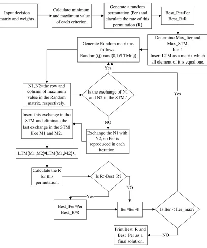
4.1. TS for APM

There are many important applications in different fields of sciences where it is practically impossible to detect the optimal solution. In such cases, one of the relevant choices is to use meta-heuristic approaches such as TS or PSO. TS was first proposed by Glover (1989, 1990) and it has been dramatically changing the ability of solving problems of practical significance. The pseudo code of the proposed TS for APM is as follows:

1. Insert decision matrix and weights, Calculate the minimum and maximum values of rating of each alternative with respect to each criterion

2. Generate a random permutation and calculate its rateR from (4), Entitle this permutation and its rate as Best_Per and Best_R, respectively

3. Set Max_Iter, Max_STM (Short Term Memory) and Iter=1, Insert LTM (Long Term Memory) as a matrix with all elements equal to 1

4. Generate Random matrix using (5):

) , (

) 1 , 0 ( )

, (

j i LTM rand j

i

Random = (5)

5. Set N1 and N2 as the row and the column of the maximum value in the Random matrix, respectively, if their exchange is in the STM go to step 4

6. Exchange N1 with N2 and set as Per and calculate the rate of this new permutation, Insert this exchange in STM and eliminate the last exchange in STM like (M1, M2)

7. LTM (M1, M2) =LTM (M1, M2) +1

8. If R>Best_R, then Best_R=R and Best_Per=Per

9. Iter =Iter +1. If Iter>Max_Iter, then the final solution is Best_R and Best_per; else go to step 4

There are two parameters in proposed TS. Max_Iter and Max_STM must be tuned before executing the procedure. The important factor in tuning these parameters is the number of alternatives (NOA). The tuning empirical formulas are expressed in consequence of some experiments by considering the NOA. Hence, the suitable performance of proposed TS can be achieved by setting these parameters

as:Max_Iter=40×NOA, Max_STM =

⎣

⎦

Input decision matrix and weights.

Calculate minimum and maximum value of each criterion.

Generate a random permutation(Per) and claculate the rate of this

permutation(R).

Generate Random matrix as follows:

Random(i,j)=rand(0,1)/LTM(i,j)

Determine Max_Iter and Max_STM.

Iter=1

Insert LTM as a matrix which all element of it is equal one.

N1,N2=the row and column of maximum value in the Random matrix, respectively.

Is the exchange of N1 and N2 in the STM?

Exchange the N1 with N2, so Per is reproduced in each

iteration.

Calculate the R for this permutation. LTM(M1,M2)=LTM(M1,M2)+1

Is R>Best_R? NO Yes

NO

Best_Per=Per

Best_R=R Is Iter < Iter_max? Yes

Yes

NO Print Best_R and

Best_Per as a final solution.

Iter=Iter+1

Best_Per=Per Best_R=R

Insert this exchange in the STM and eliminate the last exchange in the STM

like M1 and M2.

Fig. 1. Flowchart of the proposed TS

4.2. PSO for APM

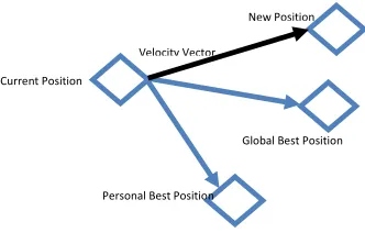
PSO is a significant member of swarm intelligence. It was proposed by Kennedy and Eberhart (1995) as a stochastic optimization method. PSO is a population based search algorithm developed based on the simulation of the social behavior of bees, birds or a school of fish. Each individual within the swarm is represented by a vector in multidimensional search space. This vector has one assigned vector which determines the next movement of the particle called the velocity vector. The PSO also determines how to update the velocity of a particle. Each particle updates its velocity based on current

velocity and the best position (p_best) it has explored so far and the global best position (g_best)

)), ( _

( . )) ( _

( . ) ( . ) 1

(t av t b₁rand p best x t b₂rand g best x t

v_i + = _i + − _i + − _i (6)

), ( ) ( ) 1

(t x t v t

x_i + = _i + _i (7)

Fig. 2. Particle movement

where i is the index of the particles, t is the index of the iteration, vi is the vector of velocity, xi is

the position, a is the inertial weight,b₁ is the weight of difference between personal best and current

position,b₂ is the weight of difference between global best and current position. Note thata , b₁

and b₂ are integer. Finally rand is used for randomization.

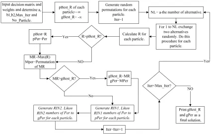
The pseudo code of the proposed PSO for APM is as follows:

1. Insert a decision matrix and weights of each criterion

2. Determine a, b1, b2, Max_Iter, and the number of particles, No_Particle, which is an integer number

3. Set pBest_R=−∞ for personal best rate of each particle andgBest_R=−∞for the global best rate, Generate random permutations for each particle and set Iter=1

4. Subtract a from the number of alternatives, for the number of the answer, exchange two alternatives randomly and repeat this step for each particle

5. Calculate the rate of each permutation R _{using Eq. (4)}, for all particles. If R>pBest_R then pBest=R and pPer=Per

6. Find the maximum rate and its permutation for this iteration, Entitle this rate and its permutation as MR and MPer, respectively. If MR>gBest_R, then gBest_R=MR and gPer=MPer

7. Generate a random integer number (RIN1) between 0 and b1. Liken RIN1 numbers of Per to pPer for each particle

8. Generate a random integer number (RIN2) between 0 and b2. Liken RIN2 numbers of Per to gPer for each particle

9. Iter=Iter+1, If Iter<Max_Iter then go to step 4; otherwise the solution is gBest_R and gPer

The flowchart of this proposed procedure is depicted in Fig. 3. There are five parameters in the proposed PSO for APM. As mentioned before, the NOA is the important factor for tuning the

parameters. Therefore, These parameters are set as: NO_Particle =15, Max_Iter=5×NOA,

1

−

=NOA

a , b₁=

⎣

⎦

⎣

⎦

1 b

b

a≥ ≥ for the implementation of our PSO and better results are normally expected using this

condition (Clerc, 2006). This procedure can also flee from the local solution by using Eq. (6) and Eq.

Velocity Vector

Current Position

Personal Best Position

Global Best Position

(7) with tuned parameters. The application and the implementation of the proposed meta-heuristics of APM are presented in the next section.

Fig. 3. Flowchart of the proposed PSO

4.3. Illustrative examples

In order to demonstrate the implementation of our proposed method we use two numerical examples in this section. The first example has 10 alternatives and 5 criteria where the second and the fifth criteria are negative attributes and the third and the fourth criteria are qualitative. The weights of the criteria are given as 0.3, 0.2, 0.1, 0.1 and 0.3, respectively. Table 2 shows the decision matrix of this example.

Table 2

Decision matrix of the first example

Criterion

Alternative 1 (+) 2 (-) 3 (+) 4 (+) 5 (-)

1 22 4.2 Very Good Medium 21

2 _{25 2.6 Good High 20}

3 _{24 1.5 Poor Low 27}

4 _{15 6.8 Good Medium 59}

5 35 7.9 Medium High 67

6 18 1.7 Poor Low 34

7 12 4.8 Very Good High 26

8 _{20 4.5 Medium Low 34}

9 _{23 3.5 Poor Medium 65}

To tackle this example, we first quantify the qualitative criteria. For the third criterion, “Poor”, “Medium”, “Good” and “Very Good” are transformed to 1, 2, 3 and 4, respectively. The fourth criterion is transformed in a similar manner. We determine the exact solution of this problem by checking all permutations and the example is solved using the two proposed meta-heuristics. The results are summarized in Table 3.

Table 3

Results of the first example

Solution method

Rank

Best rate CPU

time (s) 1 2 3 4 5 6 7 8 9 10

Exact 2 1 7 5 3 8 6 10 9 4 9.1103 557.747

TS 2 1 7 5 3 8 6 10 9 4 9.1103 0.261

PSO 2 1 7 5 3 8 6 10 9 4 9.1103 0.987

Table 3 shows that the proposed procedures replicate the solution of the exact method in a reasonable CPU time. In addition, it seems that the required CPU time for TS is less than PSO.

5. Computational experiments

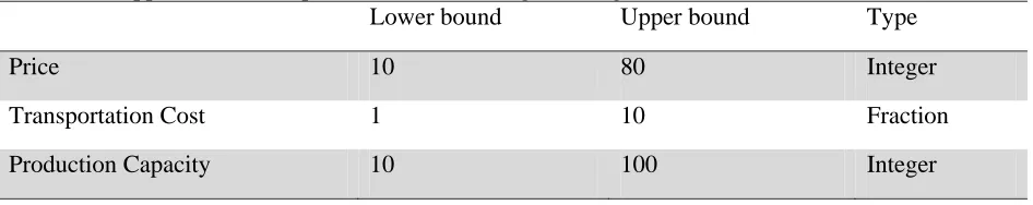
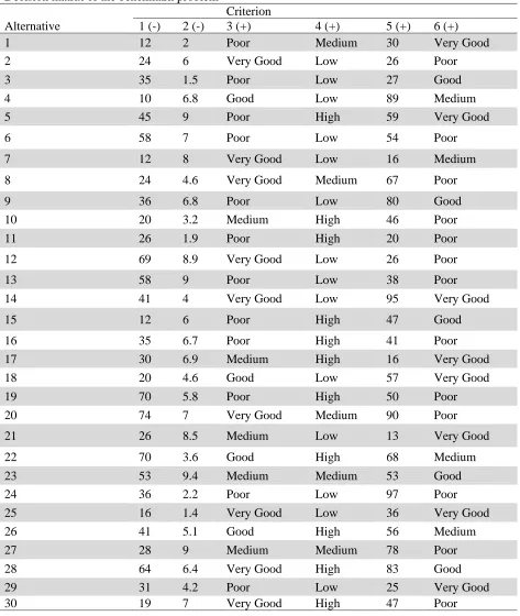
This section presents the experiments conducted to investigate the performance of TS and PSO on benchmark instances which are generated randomly. We have generated a matrix with 30 alternatives and 6 criteria. These alternatives represent the suppliers of a corporation and the criteria are price, transportation cost, delivery time, history of cooperation, production capacity and quality, respectively. To generate these random instances, lower and upper bounds are considered for each criterion. These values for the first, the second and the fifth criteria are shown in Table 4 and the other criteria are qualitative. Hence, we use similar transformation method as explained before for quantitative values. Therefore, the values can be generated randomly and 5, 10, 15, 20 and 25

alternative subsets are built by taking the top 5×6, 10×6, 15×6, 20×6 and 25×6 submatrices and we

can take 6 benchmark instances from this random problem.

Table 4

Lower and upper bounds for quantitative criteria in generating random matrix

Lower bound Upper bound Type

Price 10 80 Integer

Transportation Cost 1 10 Fraction

Production Capacity 10 100 Integer

of all permutations is impractical. This clearly calls for meta-heuristic procedures that can efficiently solve the problems.

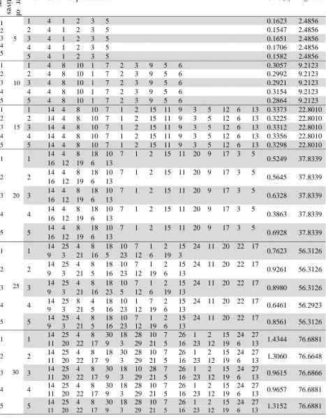
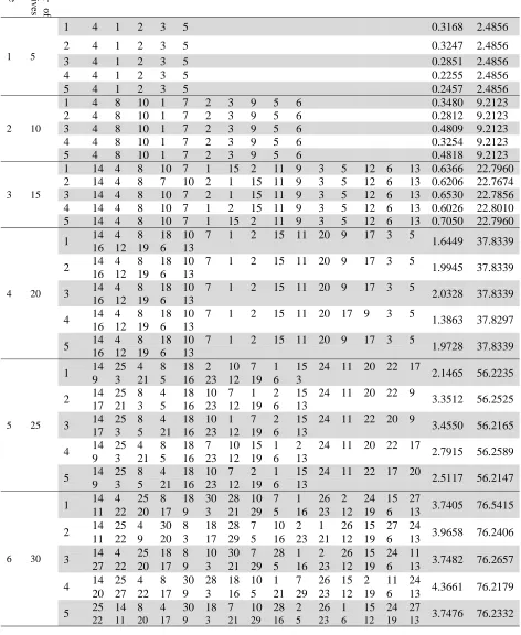
We apply the TS and PSO procedures of subsection 4.1 and 4.2 to these instances and the results are repeated five different times. Table 6 and Table 7 summarize the details of our implementations. All computations were executed using MATLAB 7.8 on a personal computer equipped with 2.99GB of RAM and a Pentium microprocessor running at 2.53 GHz.

Table 5

Decision matrix of the benchmark problem

Criterion

Alternative 1 (-) 2 (-) 3 (+) 4 (+) 5 (+) 6 (+)

1 12 2 Poor Medium 30 Very Good

2 24 6 Very Good Low 26 Poor

3 35 1.5 Poor Low 27 Good

4 10 6.8 Good Low 89 Medium

5 45 9 Poor High 59 Very Good

6 58 7 Poor Low 54 Poor

7 12 8 Very Good Low 16 Medium

8 24 4.6 Very Good Medium 67 Poor

9 36 6.8 Poor Low 80 Good

10 20 3.2 Medium High 46 Poor

11 26 1.9 Poor High 20 Poor

12 69 8.9 Very Good Low 26 Poor

13 58 9 Poor Low 38 Poor

14 41 4 Very Good Low 95 Very Good

15 12 6 Poor High 47 Good

16 35 6.7 Poor High 41 Poor

17 30 6.9 Medium High 16 Very Good

18 20 4.6 Good Low 57 Very Good

19 70 5.8 Poor High 50 Poor

20 74 7 Very Good Medium 90 Poor

21 26 8.5 Medium Low 13 Very Good

22 70 3.6 Good High 68 Medium

23 53 9.4 Medium Medium 53 Good

24 36 2.2 Poor Low 97 Poor

25 16 1.4 Very Good Low 36 Very Good

26 41 5.1 Good High 56 Medium

27 28 9 Medium Medium 78 Poor

28 64 6.4 Very Good High 83 Good

29 31 4.2 Poor Low 25 Very Good

Table 6

The proposed TS results of the benchmark instances _N

umber

o

f

alternatives

Insta

n

ces _{Run Solution permutation CPU(s) B_Rate}

1 2 3 4 5

5

1 4 1 2 3 5 0.1623 2.4856

2 4 1 2 3 5 0.1547 2.4856

3 4 1 2 3 5 0.1651 2.4856

4 4 1 2 3 5 0.1706 2.4856

5 4 1 2 3 5 0.1582 2.4856

1

10

1 4 8 10 1 7 2 3 9 5 6 0.3057 9.2123

2 2 4 8 10 1 7 2 3 9 5 6 0.2992 9.2123

3 3 4 8 10 1 7 2 3 9 5 6 0.2921 9.2123

4 4 4 8 10 1 7 2 3 9 5 6 0.3154 9.2123

5 5 4 8 10 1 7 2 3 9 5 6 0.2864 9.2123

1

15

1 14 4 8 10 7 1 2 15 11 9 3 5 12 6 13 0.3373 22.8010

2 2 14 4 8 10 7 1 2 15 11 9 3 5 12 6 13 0.3225 22.8010

3 3 14 4 8 10 7 1 2 15 11 9 3 5 12 6 13 0.3312 22.8010

4 4 14 4 8 10 7 1 2 15 11 9 3 5 12 6 13 0.3356 22.8010

5 5 14 4 8 10 7 1 2 15 11 9 3 5 12 6 13 0.3298 22.8010

1

20

1 14 4 8 18 10 7 1 2 15 11 20 9 17 3 5 0.5249 37.8339

16 12 19 6 13

2 2 14 4 8 18 10 7 1 2 15 11 20 9 17 3 5 0.5645 37.8339

16 12 19 6 13

3 3 14 4 8 18 10 7 1 2 15 11 20 9 17 3 5 0.6328 37.8339

16 12 19 6 13

4 4 14 4 8 18 10 7 1 2 15 11 20 9 17 3 5 0.3863 37.8339

16 12 19 6 13

5 5 14 4 8 18 10 7 1 2 15 11 20 9 17 3 5 0.6928 37.8339

16 12 19 6 13

1

25

1 14 25 4 8 18 10 7 1 2 15 24 11 20 22 17 0.7623 56.3126

9 3 21 16 5 23 12 6 19 3

2 2 14 25 4 8 18 10 7 1 2 15 24 11 20 22 17 0.9261 56.3126

9 3 21 5 16 23 12 19 6 13

3 3 14 25 4 8 18 10 7 1 2 15 24 11 20 22 17 0.8980 56.3126

9 3 21 16 23 5 12 6 19 13

4 4 14 25 8 4 18 10 1 7 2 15 24 11 20 22 17 0.6461 56.2923

9 3 21 5 16 23 12 19 6 13

5 5 14 25 4 8 18 10 7 1 2 15 24 11 20 22 17 0.8561 56.3126

9 3 21 5 16 23 12 19 6 13

1

30

1 14 25 4 8 30 18 28 10 7 26 1 2 15 24 27 1.4344 76.6881

11 20 22 17 9 3 29 21 5 16 23 12 19 6 13

2 2 14 25 4 8 18 30 28 10 7 26 1 2 15 24 27 1.3060 76.6648

11 20 22 17 9 3 29 21 5 16 23 12 19 6 13

3 3 14 25 4 8 30 18 10 28 7 26 1 2 15 24 27 0.9615 76.6866

11 20 22 17 9 3 29 21 5 16 23 12 19 6 13

4 4 14 25 4 8 30 18 28 10 7 26 1 2 15 24 27 0.9657 76.6881

11 20 22 17 9 3 29 21 5 16 23 12 19 6 13

5 5 14 25 4 8 30 18 28 10 7 26 1 2 15 24 27 1.3152 76.6881

Table 7

The proposed PSO results of the benchmark instances _In

st

an

ce

N

umber o

f

alter

n

at

ive

s

Run Solution permutation CPU(s) B_Rate

1 5

1 4 1 2 3 5 0.3168 2.4856

2 4 1 2 3 5 0.3247 2.4856

3 4 1 2 3 5 0.2851 2.4856

4 4 1 2 3 5 0.2255 2.4856

5 4 1 2 3 5 0.2457 2.4856

2 10

1 4 8 10 1 7 2 3 9 5 6 0.3480 9.2123

2 4 8 10 1 7 2 3 9 5 6 0.2812 9.2123

3 4 8 10 1 7 2 3 9 5 6 0.4809 9.2123

4 4 8 10 1 7 2 3 9 5 6 0.3254 9.2123

5 4 8 10 1 7 2 3 9 5 6 0.4818 9.2123

3 15

1 14 4 8 10 7 1 15 2 11 9 3 5 12 6 13 0.6366 22.7960

2 14 4 8 7 10 2 1 15 11 9 3 5 12 6 13 0.6206 22.7674

3 14 4 8 10 7 2 1 15 11 9 3 5 12 6 13 0.6530 22.7856

4 14 4 8 10 7 1 2 15 11 9 3 5 12 6 13 0.6026 22.8010

5 14 4 8 10 7 1 15 2 11 9 3 5 12 6 13 0.7050 22.7960

4 20

1 14 4 8 18 10 7 1 2 15 11 20 9 17 3 5 1.6449 37.8339

16 12 19 6 13

2 14 4 8 18 10 7 1 2 15 11 20 9 17 3 5 1.9945 37.8339

16 12 19 6 13

3 14 4 8 18 10 7 1 2 15 11 20 9 17 3 5 2.0328 37.8339

16 12 19 6 13

4 14 4 8 18 10 7 1 2 15 11 20 17 9 3 5 1.3863 37.8297

16 12 19 6 13

5 14 4 8 18 10 7 1 2 15 11 20 9 17 3 5 1.9728 37.8339

16 12 19 6 13

5 25

1 14 25 4 8 18 2 10 7 1 15 24 11 20 22 17 2.1465 56.2235

9 3 21 5 16 23 12 19 6 3

2 14 25 8 4 18 10 7 1 2 15 24 11 20 22 9 3.3512 56.2525

17 21 3 5 16 23 12 19 6 13

3 14 25 8 4 18 10 1 7 2 15 24 11 22 20 9 3.4550 56.2165

17 3 5 21 16 23 12 19 6 13

4 14 25 4 8 18 7 10 15 1 2 24 11 20 22 17 2.7915 56.2589

9 3 21 5 16 23 12 19 6 13

5 14 25 8 4 18 10 7 2 1 15 24 11 22 17 20 2.5117 56.2147

9 3 5 21 16 23 12 19 6 13

6 30

1 14 4 25 8 18 30 28 10 7 1 26 2 24 15 27 3.7405 76.5415

11 22 20 17 9 3 21 29 5 16 23 12 19 6 13

2 14 25 4 30 8 18 28 7 10 2 1 26 15 27 24 3.9658 76.2406

11 22 9 20 3 17 29 5 16 23 21 12 19 6 13

3 14 4 25 18 8 10 30 7 28 1 2 26 15 24 11 3.7482 76.2657

27 22 20 17 9 3 21 29 5 16 23 12 19 6 13

4 14 25 4 8 30 28 18 10 1 7 26 15 2 11 24 4.3661 76.2179

20 27 22 17 9 3 16 5 21 29 23 12 19 6 13

5 25 14 8 4 30 18 7 10 28 2 26 1 15 24 27 3.7476 76.2332

  5.1. Comparative Study

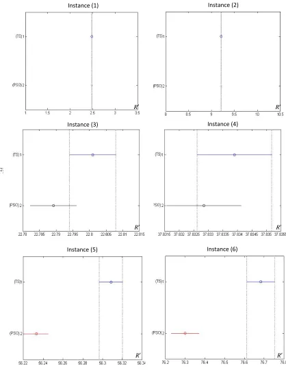
In this section we study the performance of two proposed meta-heuristic TS and PSO approaches by choosing six benchmark instances and performing ANOVA test.

Fig.

Fig. 4. ANOVA results: 95% confidence interval for the difference between TS and PSO

Instance (1)

   Instance (2)

Instance (3)

   Instance (4)

Instance (5)

   Instance (6)

R′

    R′

R′

    R′

R′

Fig. 4 summarizes the results of our investigation where the critical value for this analysis is considered as 0.05. As we can observe from Fig. 4 TS performs better compared with PSO method.

Hence, it is not necessary that the p-values of these analyses to be declared.

In the first and the second instances which represent small instances, two meta-heuristic approaches have the same results. As we explained earlier, the performance of the proposed meta-heuristics cannot be measured based on the small instances. For the third and the forth instances which represent medum size instances we could observe some differences where TS seems to perform better than PSO.

The fifth and the sixth instances represent instances for large-scale problems. As we can see from the last two instances, the two approaches in APM perform completely different. Based on the results on Table 6 and Table 7 we can conclude that TS requires less CPU time than PSO for almost all cases. The results of these tables also show that the proposed TS in APM can nearly provide the exact solution.

One other observation from the experimental results is that both meta-heuristic approaches could solve the resulted NP-Hard permutation problem in reasonable amount time for typical real-world problems. The CPU times for most large-scale problems is less than a few seconds which means that a decision maker could solve a problem different times. This could be considered as an outstanding advantage since there are many cases where we may wish to run a problem under various cicumstances to perform sensitivity analysis.

6. Conclusion

In any MADM process, there are three important criteria which need to be considered. The first one is the selection of the significant criteria. The second one is the identification of the competent alternatives and last one is to make the decision based on an effective and efficient technique. The implementation of the third one normally involves the use of some NP-Hard approaches where we need to spend significant amount of time to reach optimal solutions.

We have presented a new adjustment permutation method for permutation scheme. The proposed method of this paper has been solved using two meta-heuristic approaches of TS and PSO. The preliminary results indicate that both meta-heuristic approaches could provide reasonable solutions but the proposed TS provides better results compared with PSO for large instances. As a future research direction, we propose applying other meta-heuristic procedures such as genetic algorithm and invasive weed optimization to the APM, and comparing results of this method with other MADM techniques.

Acknowledgment

References

Ancot, J., & Paelinck, J. H. P. (1982). Recent experiences with the Qualiflex multicriteria method. in:

Paelinck, J. H. P. (Eds.), Qualitative and Quantitative Mathematical Economics., Martinus Nijhoff Publishers, pp. 217–266.

Blair, R., & Karnisky, W. (1994). Distribution-free statistical analysis of surface and volumetric

maps. Brain Topography, 6, 19–28.

Chen, T., & Wang, J. (2009). Interval-valued fuzzy permutation method and experimental analysis on

cardinal and ordinal evaluations. Journal of Computer and System Sciences, 75, 371–387.

Chin, L., & Haughton, D. (1996). Analysis of student evaluation of teaching scores using bootstrap

and permutation methods. journal of Computing in Higher Education, 8, 69–84.

Chu, T. (2002). Facility Location Selection Using Fuzzy TOPSIS under group decisions. International Journal of Uncertainty, Fuzziness and Knowledge-Based Systems, 10, 687-701.

Clerc, M.(2006). Particle Swarm Optimization. London: ISTE Ltd.

Figueira, J., Salvatore, G., Matthias, E. (2005). Multiple Criteria Decision Analysis: State of the Art

Surveys. New York: Springer Science.

Glover, F. (1989). Tabu search: Part I. ORSA Journal on Computing, 1, 190–206.

Glover, F. (1990). Tabu search: Part II. ORSA Journal on Computing, 2, 4-32.

Grabowski, J., & Pempera, J. (2007). The permutation flow shop problem with blocking. A tabu

search approach. Omega, 35, 302-311

Grabowski, J., & Wodecki, M. (2004). A very fast tabu search algorithm for the permutation flow

shop problem with makespan criterion. Computers and Operations Research, 31, 1891-1909.

Hugonnard, J., & Roy, B. (1982). Le plan d’extension du métro en banlieue parisienne, un cas type

d’application de l’analyse multicritère. Les Cahiers Scientifiques de la Revue Transports, 6, 77–

108.

Jacquet-Lagreze, E. (1969). L’agrégation des opinions individuelles. en Informatiques et Sciences

Humaines, 4, 1-21.

Kennedy, J., & Eberhart, R. (1995). Particle swarm optimization. in: Proceedings of IEEE

International Conference on Neural Networks, Piscataway, 1942–1948.

Korhonen, P., Moskowitz, H., & Wallenius, J. (1992). Multiple Criteria Decision Support: A review. European Journal of Operational Research, 63, 361-375.

Liao, L., & Huang, C. (2010). Tabu search for non-permutation flowshop scheduling problem with

minimizing total tardiness. Applied Mathematics and Computation, 217(2), 557-567.

Nowicki, E., & Smutnicki, C. (1996). A fast tabu search algorithm for the permutation flow-shop

problem. European Journal of Operational Research, 91, 160-175.

Olson, D. L. (2004). Comparison of Weights in TOPSIS Models. Mathematical and Computer

Modeling. 40(7-8), 721-727.

Peng, Y. (2000). Management Decision Analysis. Peking: Science Publications.

Paelinck, J. (1977). Qualitative multiple criteria analysis: an application to airport location. En'liironment and Planning, 9, 893–695.

Pantazis, D., Nichols, T., Baillet, S., & Leahy, R. (2003). Spatiotemporal localization of significant

activation in MEG using permutation tests. 18th Conference on Information Processing in

Medical Imaging, 512– 523.

Rinnooy K. (1976). Machine Scheduling Problems: Classification, Complexity, and Computations, Nijhoff, The Hague.

Roy, B. (1968). Classement et choix en présence de critères multiples (la method ELECTRE), RIRO,

8, 57-75.

Roy, B., & Bertier, B. (1971). Le methods ELECTRE II: Une methode de classement en presence de criteres multiples, note de travail no. 142. Direction Scientifique, Groupe Metra.

Roy, B., (1978). ELECTRE III: Un algorithme de classements fondé sur une représentation floue des

Saaty, T. L. (1990). The Analytic Hierarchy Process, McGraw-Hill, RWS Publications, Pittsburgh,

PA.

Tasgetiren, M. F., Liang, Y. C., Sevkli, M. & Gencyilmaz, G. (2007). A particle swarm optimization algorithm for makespan and total flowtime minimization in the permutation flowshop sequencing

problem. European Journal of Operational Research,177, 1930-1947.

Turskis, Z. (2008). Multi-Attribute Contractors Ranking Method by Applying Ordering of Feasible

Alternatives of Solutions in Terms of Preferability Technique. Technologic and Economic

Developement, 14, 224–239.

Yoon, K., & Hwang, C. (1981). Multiple Attribute Decision Making Method and Applications.