DEMOGRAPHIC RESEARCH
VOLUME 33, ARTICLE 19, PAGES 535–560
PUBLISHED 11 SEPTEMBER 2015
http://www.demographic-research.org/Volumes/Vol33/19/ DOI: 10.4054/DemRes.2015.33.19
Research Article
Modeling the fertility impact of the proximate
determinants: Time for a tune-up
John Bongaarts
©2015 John Bongaarts.
This open-access work is published under the terms of the Creative Commons Attribution NonCommercial License 2.0 Germany, which permits use, reproduction & distribution in any medium for non-commercial purposes, provided the original author(s) and source are given credit.
1 Introduction 536
2 Background 537
3 Proposed revisions 539
3.1 Marriage/union/sexual exposure 539
3.2 Contraception 540
3.3 Postpartum infecundability 541
3.4 Abortion 541
3.5 Model 541
4 Comparison with revisions proposed by John Stover 541 4.1 Marriage/union/sexual exposure 542
4.2 Contraception 542
4.3 Abortion 542
4.4 Postpartum infecundability 543
4.5 Sterility 543
5 Implementation of revisions 544
6 Results 546
7 Comparing the accuracy of models 553
8 Conclusion 554
9 Acknowledgements 554
References 555
Modeling the fertility impact of the proximate determinants:
Time for a tune-up
John Bongaarts1
Abstract
BACKGROUND
Many analyses of the determinants of fertility make a distinction between proximate and background determinants. The former include behavioral factors such as the use of contraception or abortion through which the background determinants (e.g., social and economic variables) affect fertility. These relationships were first recognized by Davis and Blake (1956), who defined a large set of “intermediate fertility variables.” In the late 1970s Bongaarts (1978) identified a smaller set of proximate determinants and developed a relatively simple model to quantify their fertility effects.
OBJECTIVE
This paper fine-tunes the Bongaarts proximate determinants model in light of new evidence, research, and data that have become available over the past three decades. Reproductive behavior has changed substantially and certain original simplifying assumptions have become less accurate over time. In addition, new research allows some features of the model to be improved.
METHOD
Six adjustments to the model are proposed and implemented. The revised model is compared with the original version and with a revision proposed by Stover (1998). RESULT
Revised estimates of the indexes of the proximate determinants and total fecundity are provided for the most recent DHS surveys in 36 developing countries. The revised model provides a better fit than do earlier models.
CONCLUSION
The proximate determinants model, as originally conceived, remains conceptually sound. However, theoretical and empirical evidence accumulated over the past three decades suggests a number of ways to fine-tune the model to make it more robust and accurate in contemporary populations. The resulting revised model provides an
improved assessment of the roles of the proximate determinants in national and sub-national populations.
1. Introduction
The proximate determinants (PD) of fertility are the biological and behavioral factors through which the background determinants (social, economic, and environmental variables) affect fertility. The distinguishing feature of a proximate determinant is its direct connection to fertility. If a proximate determinant, such as contraceptive use, changes, then fertility necessarily changes also (assuming the other proximate determinants remain constant). This is not necessarily true for a background determinant of fertility such as income or education. Consequently, fertility differences among populations and trends in fertility over time can always be traced to variations in one or more of the proximate determinants. If accurately measured and modeled, the proximate determinants should explain 100% of variation in fertility.
These relationships were first recognized in the mid-1950s when Kingsley Davis and Judith Blake (1956) defined a large set of proximate determinants which they called the “intermediate fertility variables.” This set was quite comprehensive and included some biological factors that differ little among populations2. In the late 1970s Bongaarts (1978, 1982) defined a somewhat different and smaller set of proximate determinants, thus simplifying the task of constructing models of human reproduction. His analysis indicated that four proximate determinants − marriage/cohabitation, contraception, induced abortion, and postpartum infecundability − are the most important for the analysis of fertility levels and trends. The identification of this smaller set of proximate determinants (PDs) led to the development of a relatively simple model that quantifies the fertility effect of each of these PDs.
The objective of this paper is to fine-tune this PD model in light of new evidence, research, and data that have become available over the past three decades. The model as originally conceived remains conceptually sound, and there is no reason to change the general multiplicative nature of the main equation. However, in recent decades reproductive behavior has changed substantially and certain original simplifying assumptions have become less accurate over time. In addition, new research allows some features of the model to be improved. A few revisions of features of the model are therefore desirable.
After a brief overview of the original PD model, the proposed revisions will be discussed and implemented. The revised model will then be applied to data from 36 developing countries using data collected in DHS surveys and compared with earlier models.
2. Background
At the core of the original PD model is the following multiplicative equation for a population at a given point in time
𝑇𝐹𝑅=𝐶𝑚𝐶𝑐𝐶𝑖𝐶𝑎𝑇𝐹
where
TFR = Observed total fertility rate
𝐶𝑚= Marriage index 𝐶𝑐= Contraception index
𝐶𝑖= Postpartum infecundability index 𝐶𝑎= Abortion index
TF = Total fecundity rate.
The model treats each PD as a factor that inhibits fertility. Each index has values that range from 1 to 0 depending on the degree of inhibition. The index of marriage 𝐶𝑚 measures the impact of the proportion of women in a marital union (i.e., formal marriage or consensual union). The index equals one when all women are cohabitating, and zero when no women are in a union. Only women in a union are assumed to be at risk of childbearing. The index 𝐶𝑐 equals one when no contraception is used, and zero when all fecund women use 100% effective contraception. The index 𝐶𝑖 equals one in the absence of lactational amenorrhea or postpartum abstinence and declines in size as the period of postpartum infecundability rises. The index of abortion equals one in the absence of abortion and declines as the incidence of abortion rises.
The total fecundity rate is the hypothetical total fertility rate that would be observed in a population in which all inhibiting effects of the proximate variables are absent, i.e., when 𝐶𝑚=𝐶𝑐 =𝐶𝑖=𝐶𝑎= 1. TF values typically are around 15 births per woman.
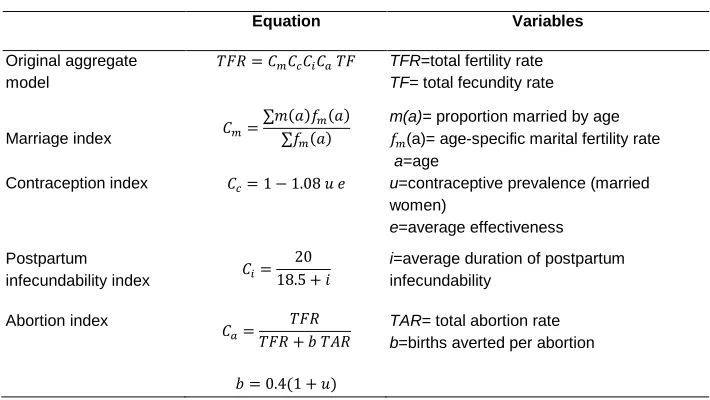
Table 1: Original aggregate proximate determinants model and equations for indexes
Equation Variables
Original aggregate model
𝑇𝐹𝑅=𝐶𝑚𝐶𝑐𝐶𝑖𝐶𝑎𝑇𝐹 TFR=total fertility rate
TF= total fecundity rate
Marriage index 𝐶𝑚=
∑𝑚(𝑎)𝑓𝑚(𝑎) ∑𝑓𝑚(𝑎)
m(a)= proportion married by age 𝑓𝑚(a)= age-specific marital fertility rate
a=age
Contraception index 𝐶𝑐= 1−1.08 𝑢𝑒 u=contraceptive prevalence (married women)
e=average effectiveness
Postpartum
infecundability index 𝐶𝑖=
20 18.5 +𝑖
i=average duration of postpartum infecundability
Abortion index
𝐶𝑎=𝑇𝐹𝑅𝑇𝐹𝑅+𝑏𝑇𝐴𝑅
𝑏= 0.4(1 +𝑢)
TAR= total abortion rate
b=births averted per abortion
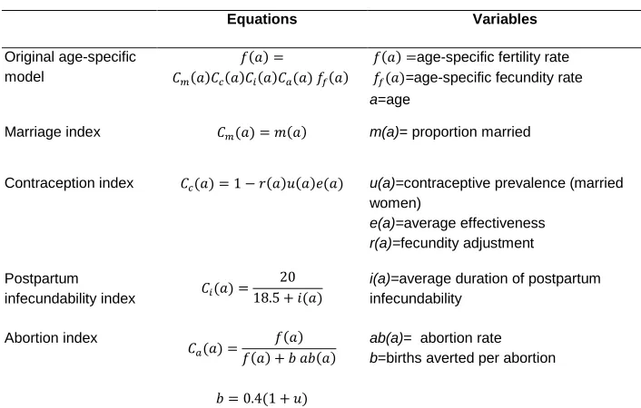
Bongaarts and Potter (1983) also proposed an age-specific version of the PD model. It is summarized in Table 2. The age-specific equations for the indexes have the same structure as those in the aggregate model in Table 1. Age specific PD models have a clear advantage over the simple aggregate models because they take account of variation in the age structures of populations (Casterline, Singh, and Cleland 1984, Hobcraft and Little 1984, Singh, Casterline, and Cleland 1985). Unfortunately, applications of age-specific models have been very limited because they are more demanding of data.
Table 2: Original age-specific proximate determinants model and equations for indexes
Equations Variables
Original age-specific model
𝑓(𝑎) =
𝐶𝑚(𝑎)𝐶𝑐(𝑎)𝐶𝑖(𝑎)𝐶𝑎(𝑎) 𝑓𝑓(𝑎)
𝑓(𝑎) =age-specific fertility rate 𝑓𝑓(𝑎)=age-specific fecundity rate
a=age
Marriage index 𝐶𝑚(𝑎) =𝑚(𝑎) m(a)= proportion married
Contraception index 𝐶𝑐(𝑎) = 1− 𝑟(𝑎)𝑢(𝑎)𝑒(𝑎) u(a)=contraceptive prevalence (married women)
e(a)=average effectiveness
r(a)=fecundity adjustment
Postpartum
infecundability index 𝐶𝑖(𝑎) =
20 18.5 +𝑖(𝑎)
i(a)=average duration of postpartum infecundability
Abortion index
𝐶𝑎(𝑎) =𝑓(𝑎) +𝑓(𝑏𝑎)𝑎𝑏(𝑎)
𝑏= 0.4(1 +𝑢)
ab(a)= abortion rate
b=births averted per abortion
3. Proposed revisions
For each of the proximate determinants, specific issues have been identified as potentially requiring a revision. These issues and the solutions proposed here to address them are as follows:
3.1 Marriage/union/sexual exposure
who are pregnant, report sex in the last month, use contraception, or are postpartum infecundable.3 In addition the name of the index of marriage will be changed to the more accurate index of sexual exposure as proposed by Stover 1998.
3.2 Contraception
As the use of contraception has risen over time, the proportion of use that overlaps with postpartum infecundability has become significant in societies with long periods of breastfeeding or abstinence (Stover 1998). Ignoring this overlap (as was done in the original model) can therefore generate inaccurate results. This is particularly the case in countries with long durations of postpartum infecundability and with family planning programs that promote contraceptive use in the early postpartum months. The solution proposed here is to exclude overlap between contraceptive use and postpartum infecundabilty in the calculation of 𝐶𝑐.
A second issue related to contraception is that the original index of contraception is derived from the prevalence of contraception among all married women aged 15-49. This assumption implies that this prevalence (and hence 𝐶𝑐) is affected by the age distribution of married women. This is inconsistent with the other indexes, which are not affected by the age distribution of the population of women in unions. The solution proposed here is to use the age-specific PD model instead of the aggregate model.
A third issue related to contraception is that the original aggregate model takes account of variations in the average level of effectiveness of contraception as affected by the method mix, but it does not explicitly account for age differences in method effectiveness (Bongaarts and Potter 1983). In contrast, the original age-specific model takes account of variation in effectiveness by age but not by method. The solution proposed here is to revise the age-specific model by allowing variation in effectiveness by age and method (see further discussion in Appendix).
3.3 Postpartum infecundability
No revisions needed (except the model-related adjustment noted below)
3.4 Abortion
The abortion index is a function of the number of births averted by an abortion. In the original formulation, this number was estimated based on the level of contraceptive prevalence with an equation that had limited analytic foundation (Bongaarts and Potter 1993). Research by Bongaarts and Westoff (2000) has examined this issue, and a more accurate equation for the number of births averted per abortion is now available (see Appendix). This new equation will be used to calculate the abortion index in the revised model proposed here.
3.5 Model
The original model assumes that the proximate determinants at a point in time affect fertility at the same time. In reality, there is a nine-month delay between a change in a proximate determinant and its impact on fertility. In addition, the DHS surveys typically measure fertility for a three-year period before the survey (i.e., on average the TFR refers to 18 months before the survey). As a result there is a mismatch of 18+9 months between the timing of the measurement of the proximate determinants at the time of the survey and the TFR. This produces significant discrepancies in countries with rapidly rising contraceptive prevalence. To address this issue, the TFR based on births 3 years before the survey will be compared with PDs measured 27 months before the date of the survey in the applications presented below.
4. Comparison with revisions proposed by John Stover
4.1 Marriage/union/sexual exposure
The two sets of revisions agree on the need to take into account sexual activity outside formal unions. However, the implementation of these revisions differs slightly. JS calculates the sexual activity index from the proportion of all women who have had sex in the last month or are pregnant or abstaining postpartum, but excludes married women who don’t meet these criteria. In contrast, JB assumes that all women who are married or in a union are exposed to the risk of pregnancy, and includes all women (regardless of their marital status) who have had sex in the last month or are pregnant or abstaining postpartum or are contraceptive users. This slightly more inclusive definition of exposure is based on the assumption that most women who are in union and have sex less than once per month still should be considered at risk of pregnancy. It also seems plausible to assume that most contraceptive users are sexually active, even if not in the past month.
In several Asian and North African surveys, no information was collected from never-married women in the latest DHS. As a result, sexual exposure in these countries is underestimated to the extent that there is extramarital exposure. These countries will not be included in the empirical analysis below.
4.2 Contraception
The two sets of revisions agree on the need to address the overlap between postpartum amenorrhea and contraceptive use, but the implementation of these revisions also differs slightly. JS excludes overlap between contraceptive use and postpartum amenorrhea. JB excludes overlap between contraceptive use and postpartum infecundability, which may be due to either breastfeeding or abstinence.
Another significant JS revision involves the fecundity adjustment to the index of contraception. This issue is discussed below and in the Appendix.
4.3 Abortion
JS proposes a slight revision to the original equation for Ca to take account of
contraceptive effectiveness. In contrast, the JB revision of Ca relies on the analysis of
4.4 Postpartum infecundability
JS and JB are in agreement, except that the latter takes into account the average 27-month delay between a change in postpartum infecundability and its impact on fertility.
4.5 Sterility
JS introduces a revised index of sterility Cf which is calculated as 1.0 minus the
proportion of sexually active women estimated to be infecund. A woman is considered infecund at the time of a survey if she is not menopausal, postpartum amenorrheic, or pregnant; has not given birth in the last five years; has not used a contraceptive and has been in a union during that period. Women who declare themselves to be infecund are also included. This is the approach used by the DHS.
1990s and later4. There seems, therefore, to be no need to introduce a sterility index to help explain variation in fertility in contemporary populations.
It should be noted that the sterility index proposed by JS shows surprising and unexplained variation among populations. For example, the proportion of sexually active women who are infecund in Asian countries is much higher than in Latin American countries (Stover 1998). There is no direct evidence that pathological sterility is higher in Asia than in Latin America. It is more plausible to assume that these differences are attributable to errors in the DHS calculations of infecundity or to the inaccurate reporting of several of the survey questions needed to estimate infecundity.
In sum, JS and JB are in broad agreement on a number issues − the revisions to include extramarital sexual exposure and to exclude overlap between contraceptive use and postpartum infecundability − even though implementations differ somewhat. But they have differing views on the usefulness of a sterility index. In addition, JB includes model changes not proposed by JS, such as the age weighting of contraceptive prevalence in the index of contraception, which is necessary to make the model analytically sound.
5. Implementation of revisions
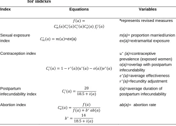
Table 3 presents the revised equations for the age-specific PD model. The calculation of these indexes requires the following age-specific variables:
m(a)= proportion married/in union ex(a)= extramarital sexual exposure
u(a)= contraceptive prevalence (among sexually active women)
o(a)= contraceptive prevalence that overlaps with postpartum infecundability e(a)= average contraceptive effectiveness
r(a)= fecundity adjustment
i(a)= average duration of postpartum infecundability f(a)= fertility rate
fm(a)=f(a)/(m(a)+ex(a))= fertility rate among sexually exposed women
ab(a)= abortion rate
All but two of these variables can be estimated from DHS surveys using procedures described by Bongaarts and Potter (1983). The exceptions are r(a), and ab(a), which require some further discussion, provided in the Appendix.
Table 3: Revised age-specific proximate determinants model and equations for indexes
Index Equations Variables
𝑓(𝑎) =
𝐶𝑚∗(𝑎)𝐶𝑐∗(𝑎)𝐶𝑖∗(𝑎)𝐶𝑎∗(𝑎) 𝑓𝑓∗(𝑎)
*represents revised measures
Sexual exposure
index 𝐶𝑚∗(𝑎) =𝑚(𝑎)+ex(a)
m(a)= proportion married/union
ex(a)=extramarital exposure
Contraception index
𝐶𝑐∗(𝑎) = 1− 𝑟∗(𝑎)(𝑢∗(𝑎)− 𝑜(𝑎))𝑒∗(𝑎)
𝑢∗ (a)=contraceptive prevalence (exposed women)
o(a)=overlap with postpartum infecundability
𝑒∗(a)=average effectiveness 𝑟∗(a)=fecundity adjustment Postpartum
infecundability index 𝐶𝑖
∗(𝑎) = 20
18.5 +𝑖(𝑎)
i(a)=average duration of postpartum infecundability
Abortion index
𝐶𝑎∗(𝑎) =𝑓(𝑎) +𝑓(𝑏𝑎∗)𝑎𝑏(𝑎)
𝑏∗= 14
18.5 +𝑖(𝑎)
ab(a)= abortion rate
*represents revised measures
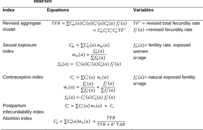
Table 4: Revised aggregate proximate determinants model and equations for indexes
Index Equations Variables
Revised aggregate model
𝑇𝐹𝑅=∑𝐶𝑚∗(𝑎)𝐶𝑐∗(𝑎)𝐶𝑖∗(𝑎)𝐶𝑎∗(𝑎) 𝑓𝑓∗(𝑎)
=𝐶𝑚∗𝐶𝑐∗𝐶𝑖∗𝐶𝑎∗𝑇𝐹∗
𝑇𝐹∗= revised total fecundity rate 𝑓𝑓∗(𝑎) =revised fecundity rate
Sexual exposure index 𝐶𝑚∗ =∑𝐶𝑚∗(𝑎) 𝑤𝑚(𝑎) 𝑤𝑚(𝑎) = 𝑓𝑚 ∗(𝑎) ∑𝑓𝑚∗(𝑎) 𝑓𝑚∗(𝑎) = 𝐶𝑐∗(𝑎)𝐶𝑖∗(𝑎)𝐶𝑎∗(𝑎) 𝑓𝑓∗(𝑎)
𝑓𝑚∗(𝑎)= fertility rate, exposed women
a=age
Contraception index 𝐶𝑐∗=∑𝐶𝑐∗(𝑎) 𝑤𝑐(𝑎)
𝑤𝑐(𝑎) = 𝑓𝑛 ∗(𝑎) ∑𝑓𝑛∗(𝑎)≈ 𝑓𝑓∗(𝑎) ∑𝑓𝑓∗(𝑎) 𝑓𝑛(𝑎) =𝐶𝑖∗(𝑎)𝐶𝑎∗(𝑎) 𝑓𝑓∗(𝑎)
𝑓𝑛∗(𝑎)= natural exposed fertility a=age Postpartum infecundability index 𝐶𝑖∗=∑𝐶𝑖∗(𝑎) 𝑤𝑖(𝑎) ≈ 𝐶𝑖 Abortion index 𝐶𝑎∗=∑𝐶𝑎∗(𝑎)𝑤𝑎(𝑎) ≈𝑇𝐹𝑅𝑇𝐹𝑅+𝑏∗𝑇𝐴𝑅
*represents revised measures
6. Results
Estimates of each of the revised indexes were obtained from data collected in the latest available DHS surveys in 36 countries. Countries are limited to those that have at least two standard all-women DHS surveys (to allow interpolation of the proximate determinants) and ex-Soviet countries are excluded.5 Given the significant revisions proposed here, it is of interest to briefly examine the differences between the three models being examined here (i.e., the original version and the revisions by JS and JB).
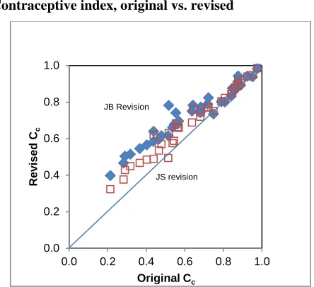
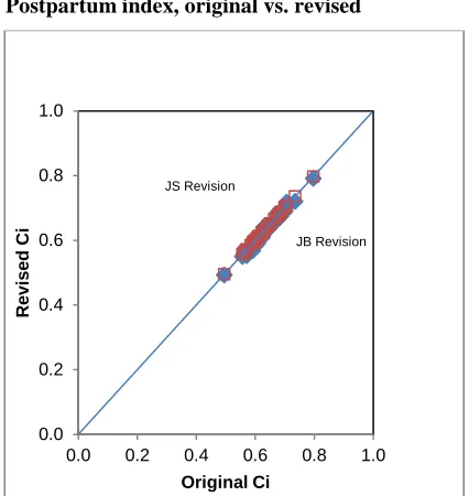
Figures 1 to 4 plot the JS and JB indexes versus the original indexes. As expected, the three sets of indexes are positively correlated. The strongest correlations are observed for Cc, Ci,and Ca, and the weakest for Cm. The latter finding is in part due to
an outlier, Namibia, where extramarital sex is relatively common. Namibia’s original
value for Cm equaled 0.30 while the JC and JB revised values for Cm equal 0.51 and
0.74 respectively.
Figure 1: Sexual exposure index, original vs. revised
Figure 2: Contraceptive index, original vs. revised 0.0
0.2 0.4 0.6 0.8 1.0
0.0 0.5 1.0
R
evi
sed
C
m
Original Cm
JB revision
JS revision
0.0 0.2 0.4 0.6 0.8 1.0
0.0 0.2 0.4 0.6 0.8 1.0
R
evi
sed
C
c
Original Cc
JB Revision
Figure 3: Postpartum index, original vs. revised
Figure 4: Abortion index, original vs. revised 0.0
0.2 0.4 0.6 0.8 1.0
0.0 0.2 0.4 0.6 0.8 1.0
R
evi
sed
C
i
Original Ci
JS Revision
JB Revision
0.0 0.2 0.4 0.6 0.8 1.0
0.0 0.2 0.4 0.6 0.8 1.0
R
evi
sed
C
a
Original Ca
JB Revision
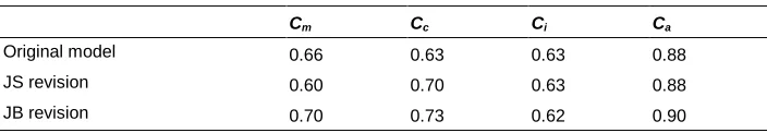
Table 5 presents the unweighted averages for the four indexes for the different models. The three models provide quite similar estimates for Ciand Ca, but differences
are substantial for Cm and Cc. Particularly notable is the difference in Cm between the JS
and the JB models (0.60 vs 0.70) which is primarily due to the way women who are married but did not have sex in the last month are treated. This group of women is excluded in the JS model but is included in the JB model. Differences in average values of Cc are also substantial. This is in part due to the exclusion of contraceptive overlap
with postpartum infecundability (which raises Cc) in the JS and JB models and to the
use of age-weighing (which also raises Cc) in the JB model6.
Table 5: Unweighted average of indexes for 36 countries
Cm Cc Ci Ca
Original model 0.66 0.63 0.63 0.88
JS revision 0.60 0.70 0.63 0.88
JB revision 0.70 0.73 0.62 0.90
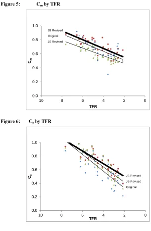
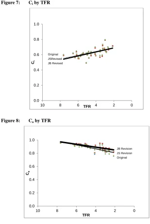
Figures 5 to 8 plot the three sets of indexes by the TFR. As expected, the indexes Cm, Cc, and Ca decline as countries move from high to low fertility and the inhibiting
effects of these PDs become stronger. In contrast, Cirises as countries move through the
transition because breastfeeding and postpartum abstinence decline. The largest differences between models are observed for Cm and Cc as expected from the findings in
Table 5. Interestingly, the slopes of the regression lines fitted to the three model estimates are similar for Cm. In contrast, the slopes for Cc vary by model, and countries
with low fertility have the largest differences between models.
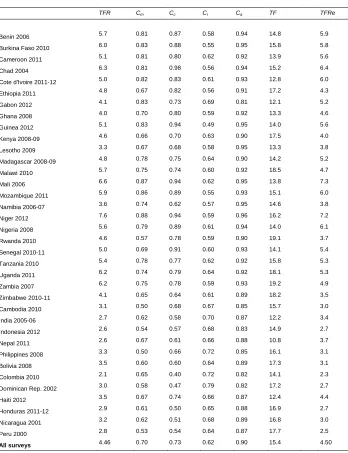
Estimates of the JB revised indexes as well as TFR and TF for individual countries are provided in Table 6. Note that the average value of TF for the 36 countries is 15.4, which is close to the estimate of 15.3 provided by Bongaarts and Potter (1983).
6
Figure 5: Cm by TFR
Figure 6: Cc by TFR 0.0 0.2 0.4 0.6 0.8 1.0
0 2
4 6
8 10
Cm
TFR
JB Revised Original JS Revised
0.0 0.2 0.4 0.6 0.8 1.0
0 2
4 6
8 10
Cc
TFR
Figure 7: Ci by TFR
Figure 8: Ca by TFR 0.0 0.2 0.4 0.6 0.8 1.0
0 2
4 6
8 10
Ci
TFR
Original JSRevised JB Revised
0.0 0.2 0.4 0.6 0.8 1.0
0 2
4 6
8 10
Ca
TFR
Table 6: Estimates of proximate determinant indexes and TFR , TF, and TFRe
for 43 DHS countries
TFR Cm Cc Ci Ca TF TFRe
Benin 2006 5.7 0.81 0.87 0.58 0.94 14.8 5.9 Burkina Faso 2010 6.0 0.83 0.88 0.55 0.95 15.8 5.8 Cameroon 2011 5.1 0.81 0.80 0.62 0.92 13.9 5.6 Chad 2004 6.3 0.81 0.98 0.56 0.94 15.2 6.4 Cote d'Ivoire 2011-12 5.0 0.82 0.83 0.61 0.93 12.8 6.0 Ethiopia 2011 4.8 0.67 0.82 0.56 0.91 17.2 4.3 Gabon 2012 4.1 0.83 0.73 0.69 0.81 12.1 5.2 Ghana 2008 4.0 0.70 0.80 0.59 0.92 13.3 4.6 Guinea 2012 5.1 0.83 0.94 0.49 0.95 14.0 5.6 Kenya 2008-09 4.6 0.66 0.70 0.63 0.90 17.5 4.0 Lesotho 2009 3.3 0.67 0.68 0.58 0.95 13.3 3.8 Madagascar 2008-09 4.8 0.78 0.75 0.64 0.90 14.2 5.2 Malawi 2010 5.7 0.75 0.74 0.60 0.92 18.5 4.7 Mali 2006 6.6 0.87 0.94 0.62 0.95 13.8 7.3 Mozambique 2011 5.9 0.86 0.89 0.55 0.93 15.1 6.0 Namibia 2006-07 3.6 0.74 0.62 0.57 0.95 14.6 3.8 Niger 2012 7.6 0.88 0.94 0.59 0.96 16.2 7.2 Nigeria 2008 5.6 0.79 0.89 0.61 0.94 14.0 6.1 Rwanda 2010 4.6 0.57 0.78 0.59 0.90 19.1 3.7 Senegal 2010-11 5.0 0.69 0.91 0.60 0.93 14.1 5.4 Tanzania 2010 5.4 0.78 0.77 0.62 0.92 15.8 5.3 Uganda 2011 6.2 0.74 0.79 0.64 0.92 18.1 5.3 Zambia 2007 6.2 0.75 0.78 0.59 0.93 19.2 4.9 Zimbabwe 2010-11 4.1 0.65 0.64 0.61 0.89 18.2 3.5 Cambodia 2010 3.1 0.50 0.68 0.67 0.85 15.7 3.0 India 2005-06 2.7 0.62 0.58 0.70 0.87 12.2 3.4 Indonesia 2012 2.6 0.54 0.57 0.68 0.83 14.9 2.7 Nepal 2011 2.6 0.67 0.61 0.66 0.88 10.8 3.7 Philippines 2008 3.3 0.50 0.66 0.72 0.85 16.1 3.1 Bolivia 2008 3.5 0.60 0.60 0.64 0.89 17.3 3.1 Colombia 2010 2.1 0.65 0.40 0.72 0.82 14.1 2.3 Dominican Rep. 2002 3.0 0.58 0.47 0.79 0.82 17.2 2.7 Haiti 2012 3.5 0.67 0.74 0.66 0.87 12.4 4.4 Honduras 2011-12 2.9 0.61 0.50 0.65 0.88 16.9 2.7 Nicaragua 2001 3.2 0.62 0.51 0.68 0.89 16.8 3.0 Peru 2000 2.8 0.53 0.54 0.64 0.87 17.7 2.5
7. Comparing the accuracy of models
A common approach to assess the accuracy of PD models is to compare the observed TFR with a model estimated TFRe in a set of countries (Bongaarts and Potter 1983,
Stover 1998). The value of TFRe in a country is obtained by a three step process: 1)
calculate the total fecundity rate (TF) by dividing the observed TFR by the product of all indices, 2) average the values of TFs in a group of countries (36 in the present study) to obtain TFave and 3) multiply TFave by the product of all country specific indices to obtain 𝑇𝐹𝑅𝑒. That is, for the original and JB models
𝑇𝐹𝑅𝑒=𝐶𝑚∗𝐶𝑐∗𝐶𝑖∗𝐶𝑎∗ 𝑇𝐹𝑎𝑣𝑒
The JS model has a similar equation, but differs slightly because it has different subscripts for the indexes, and it includes a fifth index of sterility7 (see Stover 1998 for details). Despite these differences, the process for estimating 𝑇𝐹𝑅𝑒 is the same.
The results of this comparison are summarized in Table 7. The first and second rows of this table present the unweighted averages of the observed and model-estimated total fertility rates for the 36 countries. The average error in the estimates (i.e., TFRe-
TFR) in the third row gives the bias for the models. A perfect model would have no bias. Instead, the results show that all three models have a positive bias ranging from 1.19 (births per woman) for the original model to 0.04 for the JB model. A second indicator of the accuracy of the model is the standard deviation of the error which is presented in the last row of Table 7. In a perfect model, this standard deviation would be zero. In the populations examined here, the standard deviation of the error is positive with the largest value (1.47) for the original model and the lowest (0.61) for the JB model. It should be noted that both the JS and JB revised models perform much better than the original model, in part due to a few outliers such as Namibia. In addition, the JB model is somewhat more accurate than the JS model according to the measures used in Table 6.
Table 7: Unweighted average of observed and model estimates of total fertility rates for 36 countries and mean and standard deviation of error
Original (Bongaarts)
JS revision (Stover)
JB revision (Bongaarts)
Observed TFR 4.46 4.46 4.46
Model estimated TFRe 5.65 4.64 4.50
Error (TFRe- TFR) 1.19 0.18 0.04
Standard deviation of error 1.47 0.76 0.61
But none of the models is perfect. There are several possible explanations for the differences between TFR and TFRe in all three models:
1) Errors in the estimates of the TFR (both sampling and non-sampling) 2) Errors in measures of the proximate determinants
3) Errors in the model equation for estimating the indexes and TF
4) True variation in TF due to differences in frequency of intercourse and sterility.
Unfortunately, it is not possible to quantify the roles of these potential errors.
8. Conclusion
The original proximate determinants model developed in the late 1970s by Bongaarts has found wide use in the analysis of levels, differentials, and trends in fertility. Theoretical and empirical evidence accumulated over the past three decades suggests a number of ways to fine-tune the model to make it more robust and accurate in contemporary populations. Six adjustments are proposed and implemented in this study. Compared with the original model and the revisions proposed by Stover (1998), the resulting new revised model provides an improved assessment of the roles of the proximate determinants, as indicated by a greater accuracy in predicting the TFR in a group of 36 countries with recent DHS surveys. The aggregate version of the revised model is directly derived from the age-specific model, which provides a sounder analytic basis for estimating the fertility impact of the proximate determinants. This is particularly the case for applications to sub-national populations (e.g., level of education or urban-rural) because differences in age structures can be substantial.
9. Acknowledgements
References
Blanc, A. (2004). The role of conflict in the rapid fertility decline in Eritrea and prospects for the future. Studies in Family Planning 35(4): 236–245.
doi:10.1111/j.0039-3665.2004.00028.x.
Bongaarts, J. (1978). A framework for analyzing the proximate determinants of fertility. Population and Development Review 4(1): 105–132. doi:10.2307/1972149.
Bongaarts, J. (1982). The fertility-inhibiting effects of the intermediate fertility variables. Studies in Family Planning 13(6/7): 178–189.
Bongaarts, J. and Kirmeyer, S. (1982). The relationship between prevalence of contraceptive use and fertility. In: Hermalin, A. and Entwisle, B. (eds.). The Role of Surveys in the Analysis of Family Planning Programs. Liège, Belgium: Ordina Editions.
Bongaarts, J. and Potter, R. (1983). Fertility, Biology, and Behavior: An Analysis of the Proximate Determinants. New York: Academic Press. doi:10.1016/B978-0-08-091698-9.50006-3.
Bongaarts, J. and Westoff, C. (2000). The potential role of contraception in reducing abortion. Studies in Family Planning 31(3):193–202. doi:10.1111/j.1728-4465.2000.00193.x.
Casterline, J.B., Singh, S. and Cleland, J. (1984) The proximate determinants of fertility. WFS Comparative Studies no. 39. Voorburg, Netherlands: ISI.
Caraël, M., Cleland, J., Deheneffe, J–C., Ferry, B., and Ingham, R. (1995) Sexual behaviour in developing countries: implications for HIV control. AIDS 9(10):1171–5.
Davis, K. and Blake, J. (1956). Social structure and fertility: An analytic framework. Economic Development and Cultural Change 4(3): 211–235. doi:10.1086/4497 14.
Hobcraft J. and Little, R.J.A. (1984) Fertility Exposure Analysis: A New Method for Assessing the Contribution of Proximate Determinants to Fertility Differentials. Population Studies 38(1): 21–45. doi:10.1080/00324728.1984.10412821.
Fortson, J. (2009) HIV/AIDS and Fertility. American Economic Journal: Applied Economics 1(3):170–194.
Frank, O. (1983). Infertility in sub-Saharan Africa: Estimates and implications. Population and Development Review 9(1): 137-144. doi:10.2307/1972901. Institute of Medicine. (1995). The Best Intentions: Unintended Pregnancy and the
Well-Being of Children and Families. Committee on Unintended Pregnancy, Division of Health Promotion and Disease Prevention. Sarah S. Brown and Leon Eisenberg (eds). Washington, D.C.: National Academy Press.
MacQuarrie, K.L.D. (2014). Unmet Need for Family Planning among Young Women: Levels and Trends. DHS Comparative Reports No. 34. Rockville, Maryland, USA: ICF International.
Sedgh, G., Bankole, A., Singh, S., and Eilers, M. (2012a). Legal abortion levels and trends by woman’s age at termination. International Perspectives on Sexual and Reproductive Health 38(3):143–53. doi:10.1363/3814312.
Sedgh, G., Singh S., Shah, I., Åhman, E., Henshaw S., and Bankole, A. (2012b). Induced abortion: Incidence and trends worldwide from 1995 to 2008. The Lancet 379(9816): 625–632. doi:10.1016/S0140-6736(11)61786-8.
Singh, S., Casterline, J.B., and Cleland, J.G. (1985). The Proximate Determinants of Fertility: Sub-national Variations. Population Studies 39(1): 113–135.
doi:10.1080/0032472031000141316.
Stover, J. (1998). Revising the proximate determinants of fertility framework: What have we learned in the past 20 years? Studies in Family Planning 29(3): 255– 267. doi: 10.2307/172272.
Appendix: Procedures for estimating variables and parameters
1. Births averted per abortion
An analysis of the tradeoff between abortion and contraception by Bongaarts and Westoff (2000) estimates the number of births averted per abortion as the ratio of the average reproductive time associated with an abortion to the average reproductive time associated with a live birth. Following Bongaarts and Potter (1983), the former can be estimated as 14 months and the latter as 18.5 plus the average postpartum infecundability interval. The revised equation for the number of births averted per abortion therefore is
𝑏∗= 14
18.5+𝑖 (A1)
In theory, this equation should allow for variation in i by age in the age-specific version of the revised model. But in practice the postpartum infecundability interval rises only slightly by age, and the other components of birth and abortion intervals also rise as the waiting time to conception increases with age. The net result is only a small variation in b* by age, and in the applications in this study b* and i will be given the average value at all ages.
2. Age-specific abortion rates
In developed countries with reasonably accurate abortion statistics, abortion rates by age have an inverted U graph-shape, with peak rates between ages 20 and 29 (Sedgh et al. 2012a). For present purposes it will be assumed that the countries included in this paper also have an inverted U graph-shape. Given the absence of accurate age data for abortion rates, it will further be assumed that this shape (but not the level) is the same as that of the specific fertility rates. With this simplifying assumption, the ratio of age-specific abortion rates to age-age-specific fertility rates is equal to TAR/TFR at all ages. As a result, 𝐶𝑎∗(𝑎) =𝐶𝑎∗.
et al. (2012b). The exception is Gabon, for which country estimates are available from other sources.8
3. Fecundity adjustment factor r(a)
The parameter r(a) adjusts the prevalence of contraceptive use among all exposed women to account for the fact that prevalence is higher among fecund women than among infecund women. To estimate this parameter, a slightly revised version of a method developed by Bongaarts and Kirmeyer (1982) is applied. The method starts by introducing a new variable 𝑓𝑛𝑐(𝑎) which is defined as the fertility rate of exposed women that would be observed in the absence of abortion and postpartum infecundability. As a result
𝑓𝑛𝑐(𝑎) = 𝐶𝑚∗(𝑎)𝑓𝐶(𝑎)
𝑖∗(𝑎)𝐶𝑎∗(𝑎) (A2)
=𝑓𝑓∗(𝑎)𝐶𝑐∗(𝑎) (A3) =𝑓𝑓∗(𝑎) [1− 𝑟∗(𝑎)(𝑢∗(𝑎)− 𝑜(𝑎))𝑒∗(𝑎)] (A4)
In this equation 𝑓𝑛𝑐(𝑎) can be calculated with equation (A2) from estimates of
𝑓(𝑎), 𝐶𝑚∗(𝑎),𝐶𝑖∗(𝑎), and 𝐶𝑎∗(𝑎) using data from DHS surveys. The product (𝑢∗(𝑎)− 𝑜(𝑎))𝑒∗(𝑎) can also be estimated from DHS data on contraceptive prevalence and
method mix by age (and using standard estimates of effectiveness by method from Bongaarts and Potter (1983)).
The unknowns in equation (A3) are the fecundity rate 𝑓𝑓∗(𝑎) and the fecundity adjustment factor 𝑟∗(𝑎). These unknowns are estimated with a set of OLS regressions (one for each age group) as proposed by Bongaarts and Kirmeyer (1982). In each regression 𝑓𝑛𝑐(𝑎) is the dependent variable and the product (𝑢∗(𝑎)− 𝑜(𝑎))𝑒∗(𝑎) is the independent variable. These regressions yield estimates of the intercept (which estimates 𝑓̅𝑓(𝑎), the average of 𝑓𝑓∗(𝑎) for all countries) and the slope (which estimates the average impact S(a) of a unit increase in (𝑢∗(𝑎)− 𝑜(𝑎))𝑒∗(𝑎) on 𝑓𝑛𝑐(𝑎) for all countries. From these regressions 𝑟∗(𝑎) is estimated as 𝑆(𝑎) =𝑟(𝑎)𝑓𝑛(𝑎) . The regression results are shown in table A1.
Table A1: Results of OLS regression of 𝒇𝒏𝒄(𝒂) on (𝒖∗(𝒂)− 𝒐(𝒂))𝒆∗(𝒂)
15–19 20–24 25–29 30–34 35–39 40–44 45–49
Intercept𝑓̅𝑓(𝑎) 679 631 588 514 380 192 60
Slope S(a) -416 -516 -586 -546 -409 -224 -88
𝑟∗(𝑎) =𝑆(𝑎)/ 𝑓̅
𝑓(𝑎) 0.62 0.81 0.99 1.08 1.14 1.26 1.62
The above values of 𝑓̅𝑓(𝑎) and 𝑟∗(𝑎) are used in the calculations of the model index
𝐶𝑐∗(𝑎).
Note that the fecundity adjustment 𝑟∗(𝑎) is lower than one in age group 15-19 and 20-24. This finding is explained by the fact that e(a) as calculated from the method mix does not include the effect of age on method effectiveness (e.g. because method effectiveness among spacers is lower than among limiters). The above estimate of
𝑟∗(𝑎) therefore also picks up the effects of age on method effectiveness. Since the
youngest age groups have below-average method effectiveness, the value of 𝑟∗(𝑎) falls below 1. At higher ages the shape of the 𝑟∗(𝑎) function is similar to the one estimated by Bongaarts and Kirmeyer (1982).
To check the plausibility of the age patterns of the indexes, estimates of age-specific fecundity rates were calculated for all countries with
𝑓𝑓∗(𝑎) = 𝐶 𝑓(𝑎)
𝑚∗(𝑎)𝐶𝑐∗(𝑎)𝐶𝑖∗(𝑎)𝐶𝑎∗(𝑎)