JIEM, 2015 – 8(3): 1051-1068 – Online ISSN: 2013-0953 – Print ISSN: 2013-8423 http://dx.doi.org/10.3926/jiem.1365
A Distribution-Free Newsvendor Model with
Balking Penalty and Random Yield
Chongfeng Lan
1, 2, Huanyong Ji
1, Jing Li
31
School of Economics and Management, Beijing University of Posts and Telecommunications (China)
2
School of Economics, Fuyang Normal College (China)
3
School of Economic and Management, Tian Jin University of Technology and Education (China)
lchfym@sina.com, jihuanyong1986@126.com, smartlij@163.com
Received: December 2014 Accepted: April 2015
Abstract:
Purpose: The purpose of this paper is to extend the analysis of the distribution-free
newsvendor problem under the circumstance of customer balking, which usually occurs when
customers are reluctant to buy products if the available inventory falls below a threshold level.
Design/methodology/approach: A new tradeoff tool is provided as a replacement of the
traditional one to weigh the holding cost and the goodwill costs segment: apart from the
shortage penalty, the balking penalty is introduced. Furthermore, such research methodology is
employed in the case of random yield.
Originality/value: The incorporation of balking penalty and random yield represents an
important improvement in inventory policy performance for distribution-free newsvendor
problem when customer balking occurs and the distributional form of demand is uncertain.
Keywords: newsvendor model, distribution-free, balking penalty, random yield
1. Introduction
As a fundamental problem in stochastic inventory control, the newsvendor problem has been studied for a long time and applied in a broad array of business settings with the objective of expected profit maximization or expected cost minimization (Wu, Li, Wang & Cheng, 2009). The newsvendor problem is a classical inventory problem that is very significant in terms of both theoretical and practical considerations. The model assumes that if any inventory remains at the end of the period, a discount or disposed is used to sell it. If the order quantity is lower than the realized demand, the newsvendor forgoes some profit (Khouja, 1999). In fact, the newsvendor problem has served as a building block for numerous models in inventory management, supply chain management and coordination, yield management, scheduling, option pricing models, and many other areas. See Qin, Wang, Vakharia, Chen and Seref (2011) for a survey of various newsvendor-related models and useful suggestions for future research.
The traditional newsvendor problem assumes that the demand follows a specific distribution with the known parameters. In many practical situations, however, the true demand distribution may not be easily and accurately estimated. In this paper, we focus on the situation where the probability distribution function (pdf) F belongs to a class of pdfs Ŧ with a given mean m and a given standard deviation s. The order size decision Q based only on the
Recently, Lee and Hsu (2011) study the effect of advertising that are explored for the distribution-free newsvendor problem. They show that the optimal expenditure on advertising, the optimal order quantity and the optimal lower bound on the expected profit increase with the advertising effect parameters. Güler (2014) point out that although Lee and Hsu’s result holds in general, it requires additional assumptions. He provides the necessary and sufficient conditions on the ground of the statements of Lee and Hsu (2011). Andersson, Jörnsten, Nonås, Sandal and Ubøe (2013) focus on distribution-free newsvendor problem. By comparing the performance of the maximum entropy approach with minimax regret and Scarf’s rule on large samples of randomly drawn demand distributions, they show that the average performance of the maximum entropy approach is considerably better than either alternative, and more surprisingly, that it is in most cases a better hedge against bad results. Kamburowski (2014) reveals that the distribution-free newsvendor problem under the worst-case and best-case demand scenarios actually reduces to the standard of newsvendor problem with demand distributions that bound the allowable distributions in the sense of increasing concave order.
The existing literatures regard the goodwill cost of the newsvendor just as the shortage penalty cost. However, the research discovers not only the stockout penalty cost for the goodwill cost, but also the balking penalty cost, responsible for the penalty for the lost sales of a customer during balking. The crucial differences between these two penalties involve the following aspects: first, the balking penalty occurs when the available inventory falls below a threshold (not zero) level, while the stockout penalty occurs when the inventory falls to zero. Second, since the impact of stockout on the business goodwill will be worse than the impact of customer balking in practice, the unit stockout penalty should be larger than the unit balking penalty. It is obvious that the definition of balking penalty provides another tradeoff standard for decision-maker to make a decision. Although the balking cost is generally not easy to be estimated, it is nonetheless a real cost that should not be simply ignored. Any reasonable estimate and significant of this cost improves the accuracy and profitability of the newsvendor model.
The purpose of this research work is to extend the optimal order quantity formulas established by Liao et al. (2011) to the case where balking penalty is employed in the single product case and the random yield case. We also study the effects of shortage penalty and the balking penalty on the optimal order quantity of a distribution-free newsvendor, which have been to a great extend bypassed in the existing distribution-free single period models with balking. Furthermore, we first apply the random yield to distribution-free newsvendor model with balking.
The rest of this paper is organized as follows. In Section 2 we formulate the distribution-free newsvendor models with customer balking penalty. The optimum order quantity and the lower bound on expected profit are achieved for the single product case. The random yield case is analyzed in Section 3. In Section 4, numerical experiments are presented. Finally, conclusions and suggestions for future research are detailed in Section 5.
2. Basic Model with Balking Penalty
We are going to adapt the notations largely used in Moon and Choi (1995). The notions needed for the model is given as:
• c unit cost of the inventory item
• p the item’s unit selling price
• v unit salvage value, if an item is left unsold at the end of the sales period
• q probability of a sale during balking, 0 ≤ q ≤ 1
• Q the item’s order quantity, Q >K
• l1 unit penalty for balking, i.e., unit penalty for the lost chance of a sale when the
customer in demand balks, the inventory is less than K(K ≠ 0)
• l unit penalty for stockout, i.e., unit penalty for shortage, the inventory equals zero at this time, l >l1
• D the item’s random demand
• F the distribution function of the item’s demand, F is continuous, differentiable and strictly increasing but uncertain
• m the item’s expected demand over the sales period
• s standard deviation of the item's demand
• x+ =max {x,0} the positive part of x
The expected profit function with balking and shortage penalty, as suggested by Liao et al. (2011), based on the earlier work of Moon and Choi (1995), is
πF(Q)=
∫
0 Q−K[pD+v(Q−D)]f(D)dD+
∫
Q−K Q−K+K/θ[p(Q−K+θ(D−Q+K))+v(K−θ(D−Q+K))]f(D)dD
+
∫
Q−K+K/θ∞
[pQ−l(D−(Q−K+K/θ))]f(D)dD−cQ.
In the above expression, there is no consideration of balking penalty. As mentioned earlier, however, the balking penalty may be too significant to be disregarded in many real world circumstances. Under a balking penalty situation, the lost phenomenon is different from the case presented by Liao et al. (2011). Using the above framework, we need the following expected profit function in order to incorporate the balking penalty:
πF(Q)=
∫
0 Q−K[
pD+v(Q−D)]
f(D)dD+
∫
Q−K Q−K+K/θ
[
p(Q−K+θ (D−Q+K))+v(K−θ (D−Q+K))−l1(1−θ )(D−Q+K)]
f(D)dD+
∫
Q−K+K/θ
∞
[
pQ−lθ (D−(Q−K+K/θ ))−l1(1−θ )(D−Q+K)]
f(D)dD−cQ(1)
balking does not occur. The second term denotes the expected profit if demand is between Q-K and Q–K+K/q units. In this case, balking will occur and affect (1–q)(D–(Q–K)) units
among D units demand. Thus, for this range of demand, Q–K + (D–Q+K) units will be sold and Q–(Q–K+q (D–Q+K)) units will be left unsold. So there is no stockout penalty for this case.
The balking penalty equals l1(1−q)(D−Q+K). The third term captures the expected profit when
the demand is larger than Q–K+K/q units. Now balking occurs for this case, but all items will
be sold out since the demand is large enough. Therefore, the balking penalty equals l1(1−q)
(D−Q+K) and the stockout penalty equals lq (D−(Q−K+K/q)). The last term in the above
expression represents the total cost of ordering the Q units.
Noting that
E(D−Q+K)+=
∫
Q−K ∞
(D−Q+K)f(D)dD, (2)
We can rewrite the expected profit in another form as follows (see the Appendix for the derivation):
πF(Q)=(p−v)μ−(v−v)Q−(1−θ)(p−v+l1)E(D−Q+K)+−θ(p−v+l)E(D−Q+K−K/θ)+. (3)
Remark 1
The above model (3) reduces to the profit function of the classical newsvendor problem (Gallego & Moon, 1993) when K=l=l1=0 and q =1, reduces to the model considered in Moon
and Choi (1995) when l1= l = 0, and reduces to the model considered in Liao et al. (2011)
when l1 = 0.
It is easy to verify that maximizing pF(Q) is equivalent to minimizing CF(Q), representing the total expected cost, as shown by the following expression:
CF(Q)=(c-v)Q +
(1-q)(p-v+l1)E(D-Q+K)++ q (p-v+l)E(D-Q+K-K/q)+. (4)
We can easily verify that the above expression is strictly convex in Q. Furthermore, if the exact demand distribution in (4) is known, we can find the optimal order quantity via its first partial derivative with respect to Q to zero and solving for Q, i.e.
(1-q)(p-v+l1)F(Q-K)+ q (p-v+l)F(Q-K+K/q)=p-c+q l+(1-q)l1. (5)
Let QF be the optimal order quantity obtained from (5) when the cumulative distribution of the demand is FŦ.
distributions with a finite mean m and standard deviation s. Since the distribution F of D is
unknown we want to minimize (4) against the worst possible distribution in Ŧ. To this end, we need the following results cited by Moon and Choi (1995), which are attributed to Gallego and Moon (1993):
Lemma 1
E(D−Q+K)+≤
[
σ2
+(Q−K−μ)2
]
1/2−(Q−K−μ)2 . (6)
Lemma 2
E(D−Q+K−K/θ )+
≤
[
σ2
+(Q−K−μ+K/θ )2
]
1/2−(Q−K−μ +K/θ )
2 . (7)
Lemma 3
For every Q, there exist a distribution F Ŧ where the bounds (6) and (7) are tight.
In the distribution-free newsvendor problem, our aim is to find the most unfavorable distribution for each Q and then maximize the expected total profit over Q. Using the above three lemmas, the objective is to minimize the upper bound of CF(Q) which is
CF(Q).
∇CF
(Q)=(c−v)Q+(1−θ )(p−v+l1)
[
σ2
+(Q−K−μ )2
]
1/2−(Q−K−μ)
2
+θ (p−v+l)
[
σ2
+(Q−K−μ+K/θ )2
]
1/2−(Q−K−μ +K/θ )
2 .
(8)
From (8), its second partial derivative with respect to Q is
2(∇CF
(Q))
Q2 =θ (p−v+l)σ
2
[
σ2+(Q−K−μ+K/θ )2]
−3/22 +(1−θ )(p−v+l1)σ
2
[
σ2+(Q−K−μ)2]
−3/22 >0. (9)
Therefore, (8) is convex in Q and to obtain the optimal CF(Q), we only need to compute its
first partial derivative with respect to Q and set it equal to zero, which leads to the following optimality condition:
q (p-v+l)[s2+(Q-K-m+K/q)2]-1/2(Q-K-m+K/q)+(1-q)(p-v+l1)[s2+(Q-K-m)2]-1/2(Q-K-m)=
p+v+q l+ (1-q) l1-2c.
By solving Equation (10) above for Q, we, thus, find the optimal value, Q*, which is the optimal
order quantity against the worst possible distribution. The resulting maximum distribution-free expected total profit, pF(Q*), can then be computed by substituting this value into (3).
Remark 2
In order to estimate the value of information concerning the exact distributional form of demand, we follow the notion of the expected value of additional information (EVAI) suggested by Moon and Choi (1995).
pF(QF)-pF(Q*).
This is the largest amount that we would be willing to pay for the knowledge of F. This quantity can be regarded as the expected value of additional information (EVAI).
Theorem 1
The optimal order quantity Q* is an increasing function of l and l 1.
Proof. Theorem 1 can be proved taking the first partial derivatives of (10) with respect to each parameter and determining their signs.
Let
H(l,l1)=q (p-v+l)[s2+(Q-K-m+K/q )2]-1/2(Q-K-m+K/q)+
(1-q)(p-v+l1)[s2+(Q-K-m)2]-1/2(Q-K-m)-(p+v+q l+(1-q)l1-2c)=0.
(11)
Then by the Implicit Function Theorem, from (11), we have
Q✳
l =−
H(l,l1)
l /
H(l,l1)
Q✳ . (12)
By (9), we get H(l,l1)
Q✳ >0, while
H(l,l1) l =θ
{
[
σ2
+(Q−K−μ+K/θ )2
]
−1/2(Q−k−μ +K/θ )−1
}
<0.Thus
Q✳
Similarly, by H(l,l1)
l1 =(1−θ )
{
[
σ 2+(Q−K−μ)2
]
−1/2(Q−k−μ)−1}
<0 , we can easily obtainQ✳
l1 >0.
From Theorem 1, when unit penalty for stockout l and the unit penalty for stockout l1 increase,
the decision-maker should increase the order quantity because a large order quantity may increase sales and prevent shortage.
Example 1
This example is adapted from Liao et al. (2011), incorporating an additional balking penalty cost parameter. An inventory item has the following characteristics: the unit selling price is $60, the unit cost is $35, the unit lost sale cost is $25 and the unit balking penalty cost is $10, the unit salvage value is $15. The mean and standard deviation of demand are, respectively, 850 and 150 units, but the distribution form is unknown. The balking inventory level and the unit chance of a sale, respectively, are 200 units and 0.9. From Equation (10), the optimal order quantity of the distribution-free model, Q*, is calculated to be 917 units and the resulting
expected profit, pF(Q*), obtained from (3), is $16,305.
We then assume that the item’s demand is normally distributed with the same mean and standard deviation cited above. By (5), the optimal order quantity, QF, now turns out to be 930 units and, using (6), the expected total profit, pF(QF), with exact distribution information, is
computed to be $17,492. Thus the EVAI yielded by the knowledge of the exact demand distributional form is $1,187. Based on this example, it appears that our approach results in a less than 7.5% profit penalty due to a lack of knowledge about the distribution of demand.
3. The Random Yield Case
Let us now assume that the quantity ordered or produced Q is not perfect. Consider a production environment where the decision to release Q units for production results in G(Q) good units, where G(Q) is a random variable. Let us also assume that each unit ordered or produced has the same probability r, of being good. Thus, if Q is an integer, the yield G(Q) is a
binomial random variable with mean Qr and variance Qrr where r= 1-r. This model can also
be used in a non-manufacturing setting, when an order for Q units results in the delivery of exactly Q units, each of which is good with probability r. We assume that the yield G(Q) is
We are interested in determining the optimal order quantity to maximize expected profit against the worst possible distribution of the demand. The expected profit expression (3) becomes:
pF(Q) = (p-v)m-cQ+vrQ-(1-q)(p-v+l1)E(D-G(Q)+K)+-q (p-v+l)E(D-G(Q)+K-K/q)+. (13)
As before, we transform the profit maximization problem into one of cost minimization. We find it easier to minimize the expected cost
CF(Q) = (c-v
r)Q+(1-q)(p-v+l1)E(D-G(Q)+K)+-q (p-v+l)E(D-G(Q)+K-K/q)+. (14)
Since we know the distribution of G(Q), our knowledge of the distribution of D-G(Q) is more than just its mean m-Qr and its variance s2+Qrr. Thus, applying Lemma 1 to D-G(Q), we
obtain
E(D−G(Q)+K)+≤
[
σ2+Qρ ¯ρ+(ρQ−μ−K)2]
1/2−(ρQ−μ−K)
2 . (15)
E(D−G(Q)+K−K/θ )+≤
[
σ2+Qρ ¯ρ+(ρQ−μ−K+K/θ )2]
1/2−(ρQ−μ−K+K/θ )
2 . (16)
We substitute (15) and (16) into (14) to obtain the upper bound on expected cost
∇CF
(Q)=(c−vρ )Q+(1−θ )(p−v+l1)
[
σ2
+Qρ ¯ρ+(ρQ−μ−K)2
]
1/2−(ρQ−μ−K)2
+θ (p−v+l)
[
σ2
+Qρ ¯ρ +(ρQ−μ−K+K/θ )2
]
1/2−(ρQ−μ−K+K/θ )
2 .
(17)
From (17), its second partial derivative with respect to Q is
1 8ρ
2
{
(1−θ )(p−v+l1) 4σ2
− ¯ρ2+4ρ μ+¯ 4ρ¯K
[
σ2+Qρ ¯ρ+(ρQ−μ−K)2
]
3/2+θ (p−v+l) 4σ
2
− ¯ρ2+4μ ¯ρ+4K ¯ρ−4¯ρK/θ
[
σ2+Qρ ¯ρ+(ρQ−μ−K+K/θ )2
]
3/2}
. (18) It is easier to find that 4s2-r2+4rm+4rK > 0, thus if the condition (19) holds, we can verify thatis strictly convex in Q.
4s2-r2+4mr+4Kr -4rK/q> 0. (19)
When the condition (19) holds, in order to minimize the upper bound, we need to compute its first partial derivative with respect to Q and set it equal to zero, which leads to the following optimality condition:
2(c−vρ)+(1−θ)(p−v+l1)ρ
{
12
[
σ2
+Qρρ¯+(ρQ−μ−K)2
]
−1/2[
ρ¯+2(ρQ−μ−K)]
−1}
+θ(p−v+l)ρ
{
12[
σ2+Qρρ¯+(ρQ−μ−K+K/θ)2]
−1/2[
ρ¯+2(ρQ−μ−K+K/θ)]
−1}
=0.(20)
By solving Equation (20) above for Q, thus we can find the optimal value, Q0, which is the
distribution-free expected total profit, pF(Q0), can then be computed by substituting this value
into (13).
Theorem 2
The optimal order quantity is an increasing function of l and l1when (19) holds.
Proof
Theorem 2 can be proved taking the first derivatives with respect to each parameter and determining their signs as in the proof of Theorem 1.
Let
H(l,l1)=2(c−vρ )+(1−θ )(p−v+l1)ρ
{
21[
σ2+Qρ ¯ρ +(ρQ−μ−K)2]
−1/2[
¯ρ+2(ρQ−μ−K)]
−1}
+θ (p−v+l)ρ
{
12
[
σ 2+Qρ ¯ρ +(ρQ−μ−K+K/θ )2
]
−1/2[
¯ρ +2(ρQ−μ−K+K/θ )
]
−1}
=0.(21)
Then by the Implicit Function Theorem, from (21), we have
Q0
l =−
H(l,l1)
l /
H(l,l1)
Q0 . (22)
By (18) and (19), we have
H(l,l1)
Q0 >0. (23)
Since
{
[
ρ¯+2(ρQ−μ−K+K/θ)]
2
[
σ2+Qρρ¯+(ρQ−μ−K+K/θ)2]
1/2}
2
=1− 4σ
2
− ¯ρ2+4ρ¯(μ+K−K/θ)
4
[
σ2+Qρ¯
ρ+(ρQ−μ−K+K/θ)2
]
<1.We can easily obtain
H(l,l1)
l =θ ρ
{
[
¯ρ +2(ρQ−μ−K+K/θ )
]
2
[
σ2+Qρ ¯ρ+(ρQ−μ−K+K/θ )2
]
1/2−1}
<0 . (24) ThereforeQ0
Similarly, by H(l,l1)
l1 =(1−θ )ρ
{
[
¯ρ +2(ρQ−μ−K)
]
2
[
σ2+Qρ ¯ρ+(ρQ−μ−K)2
]
1/2−1}
<0. , we getQ0
l1>0.
The results for Theorem 2 and Theorem 1 are similar. However, in Theorem 2, since the effect of random yield, we add the condition (19) to ensure the uniqueness of optimal order quantity Q0. Fortunately, in general, the condition (19) easily holds in real life and it is just a sufficient
condition.
Inference 1
The optimal order quantity Q0 is a decreasing function of
r when (19) holds.
Discussion
We can use the Implicit Function Theorem to prove Inference 1 as in the proof of Theorem 1. However, it is hard to prove Inference 1 because it is difficult to judge positive or negative of ∂H(l, l1)/∂r. By intuition, the reasoning behind Inference 1 maybe that the decision-maker
should increase the order quantity in order to provide protection against defective items when the probability of good items decrease, which implies that Inference 1 holds. We explore this issue further in Section 4, where the results of our numerical experiment are reported.
Example 2
Using the data of Example 1, we assume that for each unit of Q, the probability of being good is r = 0.9. Hence the condition (19) holds. From (20), we obtain the order quantity Q0 = 991.
4. Numerical Experiments
4.1. Robustness Analysis
In order to investigate the robustness and effectiveness of our distribution-free model (without the random yield case) developed in this paper. Specifically, we randomly generate an array of 100 test problems, where each relevant parameter of these 100 samples is drawn from a uniform distribution. Table 1 shows the distributions for the date set. For modeling demand, three different distributions, viz. normal, t and uniform are adopted. The normal and t distributions each has a mean of 800 units and a standard deviation of 150 units, whereas the uniform distribution has limits of 540 and 1,060 units, i.e. a mean of 800 and a standard deviation of 150 units.
In each distributional form, we compute the optimal expected total profits by applying the known distribution and the distribution-free cases, i.e. pF(Q*) and pF(QF). To ascertain the
effectiveness of our approach, we compute the ratio of these two measures, i.e. pF(QF)/pF(Q*).
Table 2 shows the means of these ratios for the 100 cases under the three distributions. From this table, it is clear that most of the ratios are quite close to 1, which enables us to use the distribution-free ordering rule in those circumstances when it is almost impossible or rather difficult to find the actual distributional form of demand.
Data p c v K q l l1
Range [60, 120] [30, 60] [10, 30] [150, 300] [0.5, 1] [20, 30] [10, 20]
Table 1. Distributions for randomly generated parameter values
Distribution Normal Uniform t
Mean ratio 1.0691 1.0785 1.0742
Table 2. Results of comparative examples
4.2. The Effect of Penalties
Our second numerical study is geared at understanding the influences of shortage penalty l and balking penalty l1 on the optimal order quantity, Q*, under the worst possible distribution
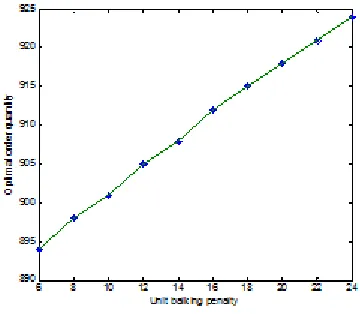
of the demand. Applying the dates of Example 1, we only need the unit shortage penalty l or the unit balking penalty l1 changes. The results of these calculations are presented in Figures
Figure 1. The influence of shortage penalty on the optimal order quantity Q*
Figure 2. The influence of balking penalty on the optimal order quantity Q*
Figure 1 and Figure 2 demonstrate that the optimal order quantity Q* is increasing in unit
shortage penalty l and in unit balking penalty l1. Therefore, when unit penalty for stockout l
and the unit penalty for stockout l1 increase, the decision-maker should increase the order
quantity in order to provide protection against balking and shortage.
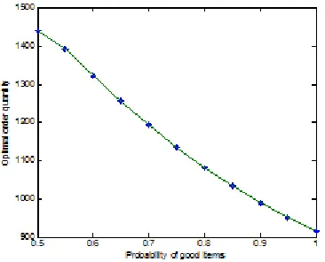
4.3. The Effect of Random Yield
Finally, the effect of random yield on the optimal order quantity, Q0, under the worst possible
Figure 3. The effect of random yield on the optimal order quantity Q0
From Figure 3, it is apparent that the optimal order quantity, Q0, is decreasing in the
probability r. Specially, the optimal order quantity reduced to 917 when r = 1, which is the
optimal order quantity without random yield case. In addition, we can experiment the inference 1 is correct by Figure 3. Therefore, the decision-maker should increase the order quantity in order to provide higher protection against defective items when the probability of good items decrease.
5. Conclusions
We have extended the distribution-free newsvendor model with customer balking developed by Moon and Choi (1995) and Liao et al. (2011), by taking the penalty for balking to the model because in real life there is always a cost associated with balking. New models and results have been accomplished for the single product case and the random yield case. We also investigate the effects of penalty for balking and shortage as well as random yield on Q* under
the worst possible distribution of the demand, which have been largely ignored in the existing distribution-free single period models with balking. Numerical results from our computational experience demonstrate the robustness and effectiveness of our enhanced model in terms of expected total profit with the comparison of the known demand distribution case. The incorporation of balking penalty and random yield, thus, represents a profound enhancement in inventory policy performance, when customer balking occurs and the distributional form of demand is unknown.
provide some insights for developing related newsvendor models with multiple ordering opportunities.
Acknowledgments
This work was supported the National Natural Science Foundation of China (71372195), the Natural Science Research Project of Anhui Province (2014KJ006), the Natural Science Research of Fuyang Normal College (2014WLGH02), and Research of Tianjin High School Social Science and Hhumanity from Tianjin Educational Committee (20142138) and Tianjin University of Technology and Education Research Foundation project (SK13-12).
References
Alfares, H.K., & Elmorra, H.H. (2005). The distribution-free newsboy problem: Extensions to the shortage penalty case. International Journal of Production Economics, 93, 465-477.
http://dx.doi.org/10.1016/j.ijpe.2004.06.043
Andersson, J., Jörnsten, K., Nonås, S.L., Sandal, L., & Ubøe, J. (2013). A maximum entropy approach to the newsvendor problem with partial information. European Journal of Operational Research, 228(1), 190-200. http://dx.doi.org/10.1016/j.ejor.2013.01.031
Cheong, T., & Kwon, K. (2013). The robust min-max newsvendor problem with balking under a service level constraint. South African Journal of Industrial Engineering, 24(3), 83-97.
http://dx.doi.org/10.7166/24-3-600
Gallego, G., & Moon, I. (1993). The distribution-free newsboy problem: Review and extensions. Journal of the Operational Research Society, 44, 825-834. http://dx.doi.org/10.1057/jors.1993.141
Güler, M.G. (2014). A note on: “The effect of optimal advertising on the distribution-free newsboy problem”. International Journal of Production Economics, 148, 90-92.
http://dx.doi.org/10.1016/j.ijpe.2013.11.021
Kamburowski, J. (2014). The distribution-free newsboy problem under the worst-case and best-case scenarios. European Journal of Operational Research, 237(1), 106-112.
http://dx.doi.org/10.1016/j.ejor.2014.01.066
Lee, C.M., & Hsu, S.L. (2011). The effect of advertising on the distribution-free newsboy problem. International Journal of Production Economics, 129(1), 217-224.
http://dx.doi.org/10.1016/j.ijpe.2010.10.009
Lee, S.W., & Jung, U. (2014). Customer balking behavior in the newsvendor model: Its impact on performance measures and decision under uncertain balking parameters. International Journal of Production Economics, 154, 274-283. http://dx.doi.org/10.1016/j.ijpe.2014.05.002
Liao, Y., Banerjee, A., & Yan, C. (2011). A distribution-free newsvendor model with balking and lost sales penalty. International Journal of Production Economics, 133(1), 224-227.
http://dx.doi.org/10.1016/j.ijpe.2010.04.024
Moon, I., & Choi, S. (1995). The distribution free newsboy problem with balking. Journal of the Operational Research Society, 537-542. http://dx.doi.org/10.1057/jors.1995.73
Moon, I., & Silver, E.A. (2000). The multi-item newsvendor problem with a budget constraint and fixed ordering costs. Journal of the Operational Research Society, 51(5), 602-608.
http://dx.doi.org/10.1057/palgrave.jors.2600938
Pal, B., Sana, S.S., & Chaudhuri, K. (2013). A distribution-free newsvendor problem with nonlinear holding cost. International Journal of Systems Science, (ahead-of-print), 1-9.
Pasternack, B.A. (1990). The newsboy problem with balking. In ORSA / TIMS Conference.
Qin, Y., Wang, R., Vakharia, A.J., Chen, Y., & Seref, M.M. (2011). The newsvendor problem: Review and directions for future research. European Journal of Operational Research, 213(2), 361-374. http://dx.doi.org/10.1016/j.ejor.2010.11.024
Scarf, H., Arrow, K.J., & Karlin, S. (1958). A min-max solution of an inventory problem. Studies in the mathematical theory of inventory and production, 10, 201-209.
Vairaktarakis, G.L. (2000). Robust multi-item newsboy models with a budget constraint. International Journal of Production Economics, 66(3), 213-226. http://dx.doi.org/10.1016/S0925-5273(99)00129-2
Wu, J., Li, J., Wang, S., & Cheng, T.C.E. (2009). Mean–variance analysis of the newsvendor model with stockout cost. Omega, 37(3), 724-730. http://dx.doi.org/10.1016/j.omega.2008.02.005
Yue, J., Chen, B., & Wang, M.C. (2006). Expected value of distribution information for the newsvendor problem. Operations research, 54(6), 1128-1136.
Appendix A.
Derivation of pF(Q)
Each term in (1) can be represented as follows:
∫
0 Q−K
[
pD+v(Q−D)]
f(D)dD−cQ=(p−v)(μ−Q+K)−(p−v)E(D−Q+K)+ (A1)∫
Q−K Q−K+K/θ
[
p(
Q−K+θ(D−Q+K))
+v(
K−θ(D−Q+K))
−l1(1−θ)(D−Q+K)]
f(D)dD=(θp−θv)E(D−Q+K)+−(θp−θv)E(D−Q+K−K/θ)+−
∫
Q−K Q−K+K/θl1(1−θ)(D−Q+K)F(D)dD
+(pQ−pK+vK)
[
1−F(Q−K)]
−pQ[
1−F(Q−K+K/θ)]
.(A2)
∫
Q−K+K/θ ∞
[
pQ−lθ(
D−(Q−K+K/θ))
−l1(1−θ)(D−Q+K)]
f(D)dD =pQ[
1−F(Q−K+K/θ)]
−lθE(D−Q+K−K/θ)+−∫
Q−K+K/θ ∞
l1(1−θ)(D−Q+K)f(D)dD. (A3)
By adding Equations (A1), (A2) and (A3) and simplifying them, we can get pF(Q) as in the text.
Journal of Industrial Engineering and Management, 2015 (www.jiem.org)
Article's contents are provided on a Attribution-Non Commercial 3.0 Creative commons license. Readers are allowed to copy, distribute and communicate article's contents, provided the author's and Journal of Industrial Engineering and Management's names are included.