Issues
ISSN: 2146-4138
available at http: www.econjournals.com
International Journal of Economics and Financial Issues, 2017, 7(5), 331-337.
The Stability of Money Demand Function in Jordan: Evidence
from the Autoregressive Distributed Lag Model
#1Adnan A. Saed
1*, Walid Al-Shawaqfeh
21Central Bank of Jordan, Jordan, 2The University of Jordan, Jordan. *Email: [email protected]
ABSTRACT
In this article, we attempt to examine the stability of real money demand function for the narrow and broad money (RM1, RM2) for the period 1995: Q1-2016: Q4 in Jordan using the autoregressive distributed lag cointegration framework. Besides the stability of real money demand, we investigate the potential long-run relationship between real demand for money and its determinants: Real gross domestic product, real interest rate, stock price index and financial development index. Empirical results based on bounds testing procedure confirm that a long-run relationship exists between real monetary aggregates (RM1, RM2) and its determinants. Moreover, most of the official monetary aggregates were used for finding out the most stable monetary demand relationship, which could provide correct signals for monetary policy formulation; the study found that narrow monetary aggregate M1 was proper aggregate. In addition, the role of financial innovation in explaining the demand for money warrants attention in formulating monetary policy. The paper imply that the central bank is able to control narrow money RM1 more accurately than broader money RM2 and could effectively use RM1 as an instrument in formulating and conducting monetary policy.
Keywords: Real Money Demand, Autoregressive Distributed Lag Model, Monetary Policy
JEL Classifications: C01, C32, O42
# The views presented in this paper are those of the authors and do not represent the views of the Central Bank of Jordan.
1. INTRODUCTION
The stability of money demand function is considered one of
the most important issues in the field of theoretical and applied
macroeconomics, because of its important implications help
economic policies and the management of monetary policy to effectively develop, and the following the behavior of money demand function and the degree of stability and its determinants increasing the effectiveness of monetary policy, the degree of
effectiveness and success of monetary policy basically depends on the extent of the stability of the money demand function, and the stability of the demand for money means the possibility to
predict the impact of the change in the money supply to some of the key economic variables such as inflation and real output and
the rate of interest and other.
It is now necessary to study the stability of the demand for money and the mechanisms of transmission of monetary impact on the Jordanian economy, specially under circumstances the economic
challenges and reform programs Jordan, where the national economy is currently facing a number of economic challenges, represents a slowdown in the economic growth in recent times; which amounted to 2.6% on average over the past 5 years; and fluctuating inflation rates; and which has seen a rise in 2008 reached 13.9%, while in 2016 amounted to a negative rate of 0.8%.
This is in addition to the exposure of the Jordanian economy to
external shocks violent the most important global financial crisis,
not to mention the increased pressure on the Jordanian economy
because of the political circumstances in the region in general and bear the burden of providing housing and public services multiple arrivals of refugees from Syria (yearly reports, Central Bank of
Jordan [CBJ]).
This study will analyze the contributions of the thought of different economic schools in determining the factors affecting the demand
for money to reach a stable function in order to enable the monetary
theory, by the contribution of classic, Keynesian and monetary
thought, in addition, technological developments and information that require to determine their effects on monetary and financial economic thought. Classical school in the crises faced by the capitalist system, the great depression analysis has failed, which led to the appearance of Keynesian thought, which appeared in the beginning of 1930th even stagflation, which opened the way
for the emergence of the monetary approach to Friedman.
The objective of this paper is to estimate the stability of real money demand function for the narrow and broad money (M1, M2) for
the period 1995: Q1-2016: Q4 in Jordan using the autoregressive distributed lag (ARDL) cointegration framework.
The rest of the paper is outlined as follows. Section 2 describes
briefly the theoretical framework for money demand. Section 3 will
provide a brief review of the literature on stability of the money demand functions. Section 4 will discuss empirical data used and
ARDL approach to cointegration. Section 5 presents some results and the final section (Section 6) concludes this study.
1.1. Monetary Policy Framework
Monetary policy development in Jordan could be perceived from
four main stages; monetary policy at the first stage which was
started since the establishment of the CBJ in 1964 and extended
to late 1980s was largely passive and the CBJ possessed little legal
or statutory independence and had only a few instruments and
limited ability to influence monetary conditions. Until 1990, the CBJ had only direct control instruments at its disposal to influence liquidity and credit conditions; including reserve requirements, liquidity ratios, directing credit to specific economic sectors, and interest rate ceilings, which led to high price distortions and non-efficiency in utilizing financial resources. These instruments were adjusted frequently to support bank liquidity and encourage credit expansion, as monetary policy was geared towards supporting the overall government policy of stimulating the economy.
After the adoption of economic reform in early 1990s, Jordan’s monetary policy stance was moving to the second stage that was
supported by the introduction of indirect control which may be
viewed as the main change in CBJ’s monetary policy. Indirect instruments represented certificates of deposits (CDs) in 1993 and open market operations (OTR) were used to influence monetary
conditions, and in 1998, the CBJ introduced another instrument
to its indirect instruments kit: It launched an overnight deposit facility, which gave the CBJ a tool for managing liquidity on a daily basis and provided a floor for inter-bank rates which increased the
ability of the CBJ to conduct monetary policy. In addition, in early
1990, the CBJ freed the credit and deposits interest rates at the banking system and let them determined in accordance to market power and competition among banks.
Initially, the CBJ was using M2 as an intermediate target to achieve its final objective of maintaining price stability and the exchange rate peg. By mid-1995, the CBJ had expanded the use of CDs to implement monetary policy and shifted to using the CD auction rate as its operational target. After 1995, the intermediate target of monetary policy changed from M2 to the banking system
interest rates, the CBJ influences the CD interest rates by varying its offerings of CDs at auction, and this would directly impact retail interest rates in the banking system. The interest rate was coincided with the change in the exchange rate peg from SDR to fixing it completely to the USD where the JD remained unchanged against the USD at the rate JD 0.709/USD until now.
In the third stage starting from 2007 until May 2012, the CBJ has moved away from solely targeting CD auction rates to a corridor system with the overnight window as the floor and the repo facility, which had been introduced in 1994, as the ceiling. In May 2007, the CBJ simplified its interest rate structure, by reducing the interest rate corridor width by 125 basis points, as it replaced the seven-day repo facility with an overnight facility to ensure symmetry with the overnight deposit window.
In May 2012, the Central Bank reviewed the monetary policy framework (the fourth stage) in two phases to meet these challenges and keep abreast of developments in the work of the central banks. The first review was in May 2012 through the
introduction of three new tools to inject liquidity into the economy,
whereby the equivalent of 2.4 billion dinars in order to influence the size of surplus reserves and control the interbank lending rate at the desired level of monetary policy through auctioning The OTR, which allows the Central Bank to intervene in the money market as a seller and purchaser of government securities, which is guaranteed by the government in order to withdraw or inject liquidity according to the requirements of the economic activity and thus helps encourage these operations in the market. And foreign currency swaps transactions in Jordanian Dinars. The Central Bank conducts foreign exchange transactions in Jordanian
Dinars with licensed banks in order to enhance the volume of liquidity in its dinar.
The second review of the operational framework of monetary
policy was in February of 2015, where the new framework gave the Central Bank sufficient flexibility in managing monetary instruments and in order to achieve the central bank’s goal of maintaining monetary stability. The focus of the development
is the adoption of a key interest rate to become the reference price for monetary policy purposes called the Central Bank interest rate, under which other interest rates for monetary policy
instruments will be set. The measure aims to give clear signals
on the position of monetary policy and its orientation towards monetary and economic developments at the domestic and external levels, and this action promotes the competition between
banks. As well as the development of liquidity management tools, enabling banks to manage their liquidity efficiently and
effectively.
Within this development, the Central Bank issued CD in dinars
for different periods and specific sizes and continued to accept bank deposits in the overnight deposit window. Within this new framework, the central bank hopes to stimulate the stagnant liquidity of banks to be exploited in achieving the objectives of economic growth through lending operations, and improve the ability of banks to manage efficient and efficient liquidity and to
2. THEORETICAL FRAMEWORK
The quantity theory of money was developed in the 19th and
early 20th century; this classical theory assumes that the money
was held for transaction purposes or as a medium of exchange.
The quantity theory of money provides an explanation how much
money in circulation and aggregate income. In addition, this theory postulates that the economy moves to a long run full-employment equilibrium. In the long run, the price level depends upon the
quantity of money in the economy. The view that interest rates do not affect the demand for money is an essential feature of this theory. The quantity theory of money equation (Fisher equation) is:
M × V = P × Y
Where:
M = Money supply V = Velocity of money
P = Price level Y = Real output.
Keynes (1936) developed the liquidity preference theory which
explicitly highlights the transaction, precautionary and speculative motives for holding money. In the Keynesian approach the assets
that can be used to store wealth are money and bonds, and the interest rate has an important effect on the money demand. The
value of money is in its purchasing power; hence the money
demand is the demand for its real value. Keynes assumed that
the real demand for money Md/P should be positively related to the real income Y and negatively related to the interest rate r, with the following general money demand function:
Md/P = f (i, Y).
Quantity theory of money by Friedman (1956) opposed the
Keynesian view that money does not matter and presented the
quantity theory as a theory of money demand and recognized
that people want and do in fact hold money for other motives.
He modelled money as abstract purchasing power (meaning that people hold it with the intention of using it for upcoming purchases of goods and services) integrated in an asset and transactions
theory of money demand set within the context of neoclassical consumer and producer behaviour microeconomic theory. It may be symbolically expressed as:
Md/P = f (Y
p, rb - rm, re - rm, πe - rm)
+ − − −
Where:
Md/P = Demand for real money balances
Yp = Present discounted value of all expected future income, or expected average long-run income, known as permanent
income
rb = Expected return on bonds rm = Expected return on money
re = Expected return on equity (common stock)
πe = Expected inflation rate.
3. EMPIRICAL STUDIES
This section includes the literature review on the empirical studies
for Jordan and other economies to modelling money demand. Bashir and Dahlan (2011) examined the money demand function in Jordan during the period (1975-2009) using the following
variables: Money supply, real income level, interest rate and
exchange rate. They estimate and test for the stability of Jordan M1 and M2 by cointegration procedure proposed by Pesaran et al. (2001) alongside CUSUM and CUSUMSQ tests. The study used
the impulse response function and the variance decomposition analysis to test the effect of determinants on money demand. The
finding indicates that there is a positive relationship between M2 and the real income level and a negative correlation between the interest rate, the exchange rate, and money demand. The stability
test revealed the stability of money demand function in Jordan.
In another study, Al-Sawaei, Zayud and Swayi (2010) examined
the determinants of narrow and broad money demand function
(M1, M2) for the period 1992-2005 and analyzed the total amount of money appropriate for use in managing monetary policy in Jordan. The research results show the existence of long-term relationship between monetary aggregates and local prices, real income and foreign interest rates.
Alyousef (2014), estimated broad money demand function (M2) in Saudi Arabia, based on ARDL model, and relying on quarterly data for the period (1996-2012). The study used the variables of real income, interest rates, index of financial innovations and stock prices. It’s found that there is a long-run stable relationship between the demand for money and its determinants. Also the
results show that all variables have a significant impact on the demand for money in the long and short term, except stock price
variable.
Al-Samara (2008), attempt to find the most important explanatory factors for the money demand in the Syrian economy using a logarithmic function, and identified the appropriate monetary transmission mechanisms and choose the intermediate goal
of monetary policy to affect prices. The results indicate that a stable money demand function and money supply helped as an
intermediate objective to influence the final goal of price stability. Kiptui (2014) examines the stability of the demand for money in Kenya by using bounds testing techniques and error correction model. The demand for broad monetary aggregates is shown to
be stable. Moreover, the real income elasticity estimates derived
in the analysis are reasonably within the range expected in the
Baumol-Tobin framework while the interest rate (Treasury
bill rate) elasticity is in the expected range of -0.1 to -0.5. The finding that demand for broad monetary aggregates is stable can be interpreted to mean that monetary targeting remains relevant
in the Kenyan context.
interest rate, effective exchange rate, inflation rate and real money
balance (M1). The results concluded that the money demand function is stable and Nigeria should effectively use money supply
as an instrument of monetary policy.
Lotfi and Ibrahim (2012) analyze the behavior of the money demand function in Egypt for the period 1991: Q1-2010: Q4. The
research attempt to test the stability of money demand function
using the cointegration procedure and error correction model, alongside with the CUSUM and CUSUMSQ stability tests. The
study concluded that there is a positive relationship between the
real income and inflation and the demand for money in the long term, and a negative relation between the interest rate and the exchange rate and the demand for money.
Halicioglu and Ugur (2005) analyse the stability of the narrow money demand function (M1) in Turkey for the period 1950-2002. They estimate and test for the stability of Turkish M1 by cointegration procedure proposed by Pesaran et al. (2001) alongside with the CUSUM and CUSUMSQ stability tests. They
demonstrate that there is a stable money demand function and
it could be used as an intermediate target of monetary policy in
Turkey.
Similarly, Chaide and Melina (2010), tested the stability of narrow money demand function relying on monthly data for the period (1989-2010) using the error correction model and the impulse response function. The findings indicate that there is instability
in the money demand function and the interest rates caused a
significant impact on the function.
Ozturk and Acaravci (2008) examined the long-run determinants of the demand for money in ten transition countries during the period (1994-2005). The paper employed the feasible generalized least squares (FGLS) model. Consistent with theoretical postulates, it is found that the demand for money in the long-run positively responds to real GDP and inversely to the inflation and the real effective exchange rate, and the long-run income elasticity is
about unity.
Finally, Kjoserski (2013) aimed to examine the short and long run
determinants and stability of money demand (M1) in Macedonia,
using monthly data from January 2005 to October 2012. Empirical results provide the evidence that exchange rate and interest rate explain most of the variation of money demand in the long run, while interest rate is significant only in the short-term. The results
also show that real money demand M1 is stable in the analyzed period.
4. DATA AND METHODOLOGY
All series examined in this study-real monetary aggregates (RM1, RM2), real gross domestic product (RGDP), real lending interest rate (RLOANR), stock price index (ASE) and financial
development index (FIND) - are collected from Central Bank of
Jordan’s statistics and International Monetary Fund bulletins over the period 1995: q1–2016: q4. All data excluding real interest rate are expressed in natural logarithm.
In this study, real monetary aggregates are used as real money demand; RGDP is used as a proxy of income, real interest rate
and stock price index are considered to be the opportunity cost for
money and financial development index for financial development (Alyousef, 2014).
In terms of methodology, the paper adopts the recently developed ARDL cointegration framework. This approach does not involve pre-testing variables, which means that the
test on the existence relationship between variables in levels
is applicable irrespective of whether the underlying regressors are purely I (0), purely I (1) or mixture of both. The ARDL model based on integration of autoregressive models with distributed lags models, and the time series is a function of its lags and values of the explanatory variables with one or more lags. (Pesaran et al., 2001)
Basically, the ARDL model for real money demand functions in
the narrow and board concept has been formulated as follows:
0 1 1 2 1 3 1
4 1 5 1 6
1
1 2
7 8
0 0
3 4
9 10 1
0 0
( 1) ( 1) ( ) ( )
( ) ( ) ( 1)
( ) ( )
( ) ( )
t t t t
p
t t t i
i
q q
t i t i
i i
q q
t i t i i
i i
RM RM RGDP RLoanr
ASE FIND RM
RGDP RLoanr ASE FIND − − − − − − = − − = = − − = = ∆ = + + + + + + ∆ + ∆ + ∆ + ∆ + ∆ +
∑
∑
∑
∑
∑
(1)0 1 1 2 1 3 1
4 1 5 1 6
1
1 2
7 8
0 0
3 4
9 10 1
0 0
( 2) ( 2) ( ) ( )
( ) ( ) ( 2)
( ) ( )
( ) ( )
t t t t
p
t t t i
i
q q
t i t i
i i
q q
t i t i i
i i
RM RM RGDP RLoanr
ASE FIND RM
RGDP RLoanr ASE FIND − − − − − − = − − = = − − = = ∆ = + + + + + + ∆ + ∆ + ∆ + ∆ + ∆ +
∑
∑
∑
∑
∑
(2)Where (RM1, RM2), (RGDP), (RLOANR), (ASE), and (FIND) are real monetary aggregates, RGDP, real interest rate, and financial development index, respectively, Δ is the first-difference operator and p is the optimal lag length. Further, lag selection was based
on Akaike Information Criterion.
The F-test is used for testing the existence of long-run relationship. When long-run relationship exists, F test indicates which variable should be normalized. The null hypothesis for no cointegration among variables in Equation (1) and Equation (2) are H0: b1 = b2
= b3 = b4 = b5 = b1 = 0. The F-test has a non-standard distribution
which depends on (i) whether variables included in the model
asymptotic critical value bounds, depending on whether the variables are I (0) or I (1) or a mixture of both. Two sets of critical values are generated with one set refers to the I (1) series and the other for the I (0) series. Critical values for the I (1) series are
referred to as upper bound critical values, while the critical values
for I (0) series are referred to as the lower bound critical values (Pesaran et al., 2001).
If the F test statistic exceeds their respective upper critical values,
we can conclude that there is evidence of a long-run relationship between the variables regardless of the order of integration of the
variables. If the test statistic is below the upper critical value, we
cannot reject the null hypothesis of no cointegration and if it lies
between the bounds, a conclusive inference cannot be made without
knowing the order of integration of the underlying regressors. The existence of a long run relationship between variables and the
short run dynamics could be express as follows:
1
0 1 2
1 0
2 3
3 4
0 0
4
5 1 1
0
( 1) ( 1) ( )
( ) ( )
( )
p q
t t i t i
i i
q q
t i t i
i i
q
t i t i
i
RM RM RGDP
RLoanr ASE FIND ECT − − = = − − = = − − = ∆ = + ∆ + ∆ + ∆ + ∆ +
∆ + Ψ +
∑
∑
∑
∑
∑
(3)
1
0 1 2
1 0
2 3
3 4
0 0
4
5 1 2
0
( 2) ( 2) ( )
( ) ( )
( )
p q
t t i t i
i i
q q
t i t i
i i
q
t i t i
i
RM RM RGDP
RLoanr ASE FIND ECT − − = = − − = = − − = ∆ = + ∆ + ∆ + ∆ + ∆ +
∆ + Ψ +
∑
∑
∑
∑
∑
(4)
All coefficients of short-run equation are coefficients relating to the short run dynamics of the model’s convergence to equilibrium and ψ is the coefficient for the error correction term (ECT), which shows the speed of convergence of the variables to its equilibrium values. The coefficient value should be significant with a negative sign.
5. RESULTS
The current paper investigates a long term dynamic relationship between real demand for money and RGDP, RLOANR, stock price index and financial development proxy (FIND) in the case of Jordan from 1995: Q1 to 2016: Q4 by using ARDL model. The results of the dynamic model are presented in the following section. 5.1. Unit Root Test
The Augmented Dickey–Fuller (ADF) test and Philips-Perron test (PP) were used to determine the presence of unit roots in the data sets. We conducted a test of order of integration for each variable
using (ADF) and (PP) tests (Table 1). Even though the ARDL framework does not require pre-testing variables to be done, the unit root test could point the usefulness of using this method. The
results in Table 1 show a mixture in order of cointegration of I (1) and I (0). Therefore, the ARDL testing could be proceeded. 5.2. Bound Test
The next step is where equation 1and 2 are estimated to examine
the long-run relationships among the variables. The calculated F-statistics for the cointegration test is displayed in Table 2. The
critical value is reported together in the same table which is based
on critical value suggested by Pesaran et al. (2001).
Table 1: Unit root tests
Variable ADF test statistic PP test statistics Level First
difference Level differenceFirst
Ln RM1 0.402 −9.909*** 0.507 −9.909***
Ln RM2 −0.027 −10.355*** 0.050 −10.393***
Ln RGDP −1.477 −3.601*** −0.895 −15.034***
RLOANR −1.444 −10.377*** −3.00**
-Ln ASE −1.862 −5.833*** −1.883 −5.842***
Ln FIND 1.021 −6.427*** −12.671***
-***Significant at 1% level, **significant at 5% level, *significant at 10% level. ADF: Augmented Dickey–Fuller, PP: Philips–Perron, RGDP: Real gross domestic product, RLOANR: Real lending interest rate
Table 2: ARDL bounds test
Model Value Significance level (%) Bound critical values I (0) I (1)
RM1 5.93 1 3.29 4.37
5 2.56 3.49
RM2 9.65 10 2.2 3.09
ARDL: Autoregressive distributed lag
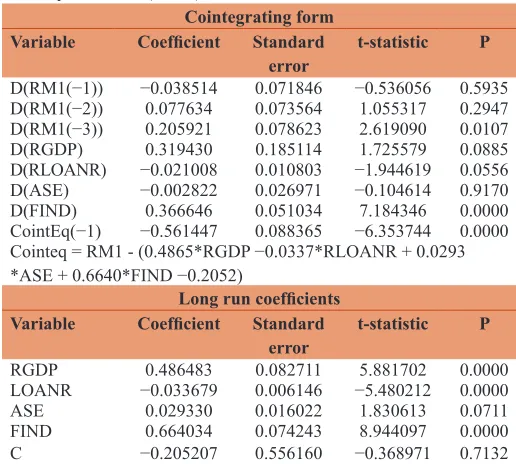
Table 3: ARDL cointegrating and long run form for real money demand (RM1)
Cointegrating form Variable Coefficient Standard
error t-statistic P D(RM1(−1)) −0.038514 0.071846 −0.536056 0.5935 D(RM1(−2)) 0.077634 0.073564 1.055317 0.2947 D(RM1(−3)) 0.205921 0.078623 2.619090 0.0107
D(RGDP) 0.319430 0.185114 1.725579 0.0885
D(RLOANR) −0.021008 0.010803 −1.944619 0.0556 D(ASE) −0.002822 0.026971 −0.104614 0.9170 D(FIND) 0.366646 0.051034 7.184346 0.0000 CointEq(−1) −0.561447 0.088365 −6.353744 0.0000 Cointeq = RM1 - (0.4865*RGDP −0.0337*RLOANR + 0.0293 *ASE + 0.6640*FIND −0.2052)
Long run coefficients
Variable Coefficient Standard
error t-statistic P
RGDP 0.486483 0.082711 5.881702 0.0000
LOANR −0.033679 0.006146 −5.480212 0.0000
ASE 0.029330 0.016022 1.830613 0.0711
FIND 0.664034 0.074243 8.944097 0.0000
C −0.205207 0.556160 −0.368971 0.7132
• The calculated F-statistic for RM1 model (F-statistic = 5.93) is higher than the upper bound critical value at 1 percent level of significance.
• The calculated F-statistic for RM2 model (F-statistic = 9.65) is higher than the upper bound critical value at 1 percent level of significance.
5.3. ARDL Model Cointegration Framework
The results of the error correction model for money demand are presented in Tables 3 and 4.
5.3.1. Real money demand model based on narrow money (RM1)
The lagged error term (ECTt−1) in our results for real money
demand (RM1) is negative and significant at 1% level. The coefficient of −0.56 indicates high rate of convergence to equilibrium. A long-run relationship was detected among real
demand for money and real income, real interest rate, stock price
index, and financial development.
5.3.2. Real money demand model based on board money (RM2)
The lagged error term (ECTt−1) in our results for real money
demand (RM2) is negative and significant at 1% level. The coefficient of −0.5 indicates low rate of convergence to
equilibrium.
Results from the Table 4 revealed a long-run relationship between
real demand for money and other variables except real interest rate.
Table 4: ARDL cointegrating and long run form for real money demand (RM2)
Co-integrating form Variable Coefficient Standard
error t-statistic P
D(RGDP) 0.308083 0.137175 2.245910 0.0281
D(LOANR) −0.017366 0.008284 −2.096455 0.0399 D(RLOANR (−1)) −0.022300 0.008565 −2.603523 0.0114 D(RLOANR (−2)) −0.032643 0.008574 −3.807064 0.0003 D(RLOANR (−3)) −0.033517 0.008730 −3.839180 0.0003 D(ASE) −0.004449 0.023174 −0.191976 0.8484 D(ASE (−1)) −0.116372 0.025110 −4.634537 0.0000 D(ASE (−2)) 0.014594 0.024353 0.599259 0.5511 D(ASE (−3)) −0.043432 0.020808 −2.087222 0.0407 D(FIND) 0.133642 0.043283 3.087639 0.0029 D(FIND (−1)) −0.179206 0.074451 −2.407038 0.0189 D(FIND (−2)) −0.136406 0.063407 −2.151280 0.0351 D(FIND (−3)) −0.109144 0.047522 −2.296694 0.0248 CointEq(−1) −0.500211 0.075514 −6.624063 0.0000 Cointeq = RM2_SA - (0.3932*RGDP −0.0099*RLOANR + 0.1024 *ASE + 0.7301*FIND + 0.0240)
Long run coefficients
Variable Coefficient Standard
error t-statistic P
RGDP 0.393209 0.121883 3.226115 0.0020
LOANR −0.009950 0.006358 −1.564803 0.1224
ASE_ 0.102424 0.027249 3.758818 0.0004
FIND 0.730116 0.109901 6.643380 0.0000
C 0.024042 0.580647 0.041406 0.9671
RGDP: Real gross domestic product, RLOANR: Real lending interest rate
Figure 1: CUSUM test (RM1 model)
Figure 2: CUSUMQ test (RM1 model)
Figure 3: CUSUM test (RM2 model)
5.4. Diagnostic Tests
We applied a number of diagnostic tests to the ARDL model. We find no evidence of serial correlation and Heteroskedasticity. The model also passes the Jarque–Bera normality test, suggesting that
errors are normally distributed (Table 5).
5.5. Testing Stability of the Demand for Money
Testing for stability of real money demand is important as real monetary aggregates is one of the key instruments of
monetary policy. If money demand is stable then money supply is the most suitable monetary policy instrument but if money demand function is instable, central bank should use another instruments for the conduct of monetary policy. To test stability, conventional methods and estimation were
used; these tests include CUSUM, CUSUMSQ and recursive
estimation technique.
As both CUSUM and CUSUMSQ statistics stay within critical
bounds at 5% level of significance, so it was the indication of the long run estimates of the demand for money function during the period 1995:Q1-2016:Q4 (Figures 1-4).
The result of the CUSUM test shows stability of the real demand
function for money (RM1, RM2) during the period (1995-2016).
Meanwhile, CUSUMQ shows stability of real money demand function (M1) and instability of the real money demand function
(M2) during the years of 2008 and 2009.
6. CONCLUSIONS AND
RECOMMENDATIONS
The purpose of this study is to investigate the stability of real
money demand function for the narrow and broad money (RM1,
RM2), and the potential long-run relationship between real demand for money and its determinants: RGDP, real interest rate, stock price index and financial development index in Jordan, using the ARDL cointegration framework.
The result of the CUSUM test show stability of the real demand
function for money (RM1, RM2) during the period (1995-2016).
Meanwhile, CUSUMQ show stability of real money demand function (M1) and instability of the real money demand function
(M2) during the years of 2008 and 2009.
The lagged error term (ECTt−1) in our results for real money
demand (RM1 and RM2) were negative and significant at 1% level. A long-run relationship was detected among real demand
for money and real income, real interest rate, stock price index,
and financial development.
The central bank is able to control narrow money RM1 more accurately than broader money RM2 and could effectively use
RM1 as an instrument in formulating and conducting monetary
policy.
REFERENCES
Al-Samara, M. (2008), Monetary Policy Analysis and its Effect in the Stability of Money Demand Function. Syria: Damascus University. Al-Sawaei, K. (2010), The Demand for Money in Jordan Using
Cointegration and Error Correction Model. Amman, Jordan: University of Jordan.
Al-Sawaei, K., Al-Zayud, K.M. (2010), The demand for money in jordan using cointegration and error correction model. Amman, Jordan: University of Jordan, Dirasat: Human and Social Science, 37, 2. Alyousef, N. (2014), Stability of money demand in Saudi Arabia. Journal
of King Saud University, 26(2), 97-110.
Bashier, A., Dahlan, A. (2011), The money demand function of Jordan: An empirical investigation. International Journal of Business and Social Science, 2, 77-86.
Central Bank of Jordan, Yearly Bulletins. (1995-2016), Monthly Statistical Bulletin. Amman, Jordan: Central Bank of Jordan.
Danele, V., Foresti, P., Napolitano, O. (2016), The stability of money demand in the long-run: Italy (1861-2011). Cliometrica, 11(2), 217-244.
Dritsaki, C., Dritsaki, M. (2012), The stability of money demand: some evidence from Turkey. The IUP Journal of Bank Management, 11(4), 7-28.
Friedman, M., editor. (1956), The quantity theory of money-a restatement. In: Studies in the Quantity Theory of Money. Chicago: The University of Chicago Press.
Halicioglu, F., Ugur, M. (2005), On stability of the demand for money in a developing OECD country: The case of Turkey. Global Business and Economics Review, 7(2-3), 203-213.
Keynes, J.M. (1936), The General Theory of Employment, Interest and Money. Vol. 7. Cambridge: MacMilan.
Kiptui, M.C. (2014), Some empirical evidence on the stability of money demand in Kenya. International Journal of Economics and Financial Issues, 4(4), 849-858.
Kjosevski, J. (2013), The determinants and stability of money demand in the republic of Macedonia. Zbornik Radova Ekonomskog Fakulteta u Rijeci, 31, 35-54.
Kumar, S., Webber, D., Fargher, S. (2010), Money Demand Stability: A Case Study of Nigeria, MPRA Paper No. 26074.
Lotfi, A., Ibrahim, E. (2012), The Stability of Money Demand Function in Developing Countries Using Cointegration and Error Correction Model: The Case of Egypt, Faculty of Trade and Finance, Tanta University.
Pesaran, M.H., Shin, Y., Smith, R.J. (2001), Bounds testing approaches to the analysis of level relationships. Journal of Applied Econometrics, 16(3), 289-326.
Walsh, C. (2010), Monetary Policy and Theory. 3rd ed. Cambridge, Massachusetts: Massachusetts Institute of Technology.
Table 5: Diagnostic tests
Model Residual
Heteroskedasticity test Residual autocorrelation LM test Residual normality test
P F-statistic P F-statistic P Jarque-Bera