shift_share_supplement.pdf

Online supplement to:

“Shift-Share Designs: Theory and Inference”

Rodrigo Adão

Michal Kolesár

Eduardo Morales

August 9, 2019

*_{University of Chicago Booth School of Business. Email:[email protected]} †_{Princeton University. Email:[email protected]}

Contents

A Proofs and additional theoretical results 4

A.1 Proofs and additional details for OLS regression . . . 4

A.1.1 General setup and assumptions . . . 4

A.1.2 Auxiliary results . . . 6

A.1.3 Proof of Proposition 3 . . . 7

A.1.4 Proof of Proposition 4 . . . 9

A.1.5 Proof of Proposition 5 . . . 12

A.1.6 Inference under heterogeneous effects . . . 15

A.2 Proofs and additional details for IV regression . . . 17

A.2.1 Assumptions . . . 17

A.2.2 Asymptotic results . . . 18

A.2.3 Proof of Proposition A.2 . . . 20

A.2.4 Proof of Proposition A.3 . . . 21

B Stylized economic model: baseline microfoundation 24 B.1 Environment . . . 24

B.2 Equilibrium . . . 26

B.3 Labor market impact of sectoral shocks: equilibrium relationships . . . 27

B.4 Identification of labor market impact of sectoral prices . . . 28

B.4.1 Impact of labor demand and supply shocks on sector-specific price indices . . . 29

C Stylized economic model: Extensions 30 C.1 Sector-specific factors of production . . . 30

C.1.1 Environment . . . 30

C.1.2 Equilibrium . . . 30

C.1.3 Labor market impact of sectoral shocks . . . 32

C.2 Sector-specific preferences . . . 33

C.2.1 Environment . . . 33

C.2.2 Equilibrium . . . 33

C.2.3 Labor market impact of sectoral shocks . . . 34

C.3 Allowing for regional migration . . . 35

C.3.1 Environment . . . 36

C.3.2 Equilibrium . . . 36

C.3.3 Labor market impact of sectoral shocks . . . 37

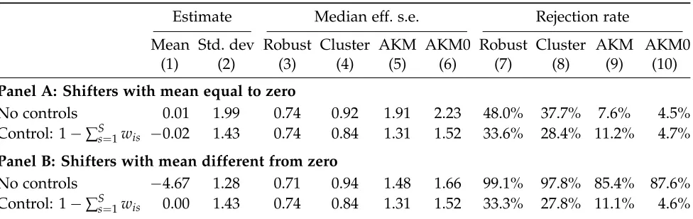
D Additional placebo exercises 39 D.1 Placebo exercise: empirical distributions. . . 39

D.2 Controlling for size of the residual sector . . . 42

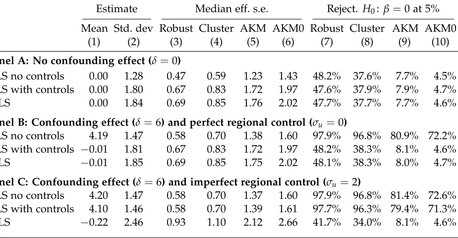
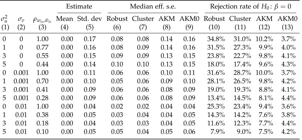
D.3 Confounding sector-level shocks: omitted variable bias and solutions . . . 42

D.5 Misspecification in linearly additive potential outcome framework . . . 48

D.5.1 Nonlinear potential outcome framework . . . 48

D.5.2 Asymptotic properties of the shift-share linear specification . . . 50

D.5.3 Simulation . . . 51

D.6 Unobserved shift-share components with different shares . . . 55

D.7 Heterogeneous treatment effects . . . 56

D.8 Other extensions . . . 57

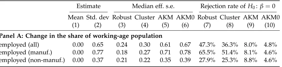
E Empirical applications: additional results 61 E.1 Effect of Chinese exports on U.S. labor market outcomes . . . 61

E.1.1 Placebo exercise: alternative distributions of shifters . . . 61

E.1.2 Placebo exercise: accounting for controls in the first-stage regression . . . 65

E.1.3 Additional empirical results . . . 65

E.2 Estimation of inverse labor supply elasticity . . . 70

E.2.1 Bias in OLS estimate of inverse labor supply elasticity . . . 70

E.2.2 Consistency of IV estimate of inverse labor supply elasticity. . . 71

E.2.3 Evaluation of leave-one-out IV through the lens of the model in Section 3 . . . . 71

E.2.4 Placebo exercise. . . 74

E.2.5 Additional results . . . 77

F Effect of immigration on U.S. local labor markets 78 F.1 Sample periods and list of countries of origin of immigrants . . . 79

F.2 Placebo simulations . . . 79

F.3 Results with a restricted set of origin countries . . . 80

Appendix A

Proofs and additional theoretical results

AppendixA.1gives proofs and additional details for the results in Sections 4.1 and 4.2. AppendixA.2

gives proofs and additional details for the results in Sections 4.3 and 5.3.

A.1 Proofs and additional details for OLS regression

Since Propositions 1 and 2 are special cases or Propositions 3 and 4, we only prove Propositions 3, 4 and 5. We give the proofs under a slightly more general setup that allows for a linearization error in the potential outcome equation. We introduce this more general setup in AppendixA.1.1, where we also collect the assumptions that we impose on the DGP. We collect some auxiliary Lemmata used in the proofs in AppendixA.1.2, and we prove these propositions in AppendicesA.1.3,A.1.3andA.1.5. AppendixA.1.6discusses inference when the effectsβis are heterogeneous.

Throughout the Appendix, we assume that ∑S_s=1wis ≤ 1 for all i. Thus, ∑Ss=1ns ≤ N, where ns = ∑iN=1wis denotes the size of sector s. We use the notation AS BS to denote AS = O(BS), i.e. there exists a constantCindependent ofSsuch thatAS≤CBS. LetF0denote theσ-field generated by (Z,U,Y(0),B,W)(for the case with no covariates,F₀ denotes theσ-field generated by(Y(0),B,W)). Definewst = ∑Ni=1wiswit, ˜Xs =Xs−Zs0γ, andσs2 =var(Xs |F0). Finally, letrN = (∑sn2s)−1, and let EW denote expectation conditional on W.

A.1.1 General setup and assumptions

We first list and discuss the regularity conditions needed for the results in Section 4.1. We then generalize the setup from Section 4.2 by allowing for a linearization error in the potential outcome equation (11). Unless stated otherwise, all limits are taken asS→∞. We leave the dependence of the number of regionsN= NSon Simplicit.

For the results in Section 4.1, we assume that the observed data (Y,X,W) is generated by the variables (Y(0),B,W,X), which we model as a triangular array, so that the distribution of the data may change with the sample size.1 The additional regularity conditions we impose on these variables, in addition to Assumptions 1 and 2 as follows:

Assumption A.1. (i) The support of β_is is bounded; (ii) _N1 ∑N_i=1∑_sS₌₁var(Xs | F0)w2_is converges in probability to a strictly positive non-random limit; (iii) For some ν > 0, E[|Xs|2+ν | F0]exists and is uniformly bounded, and conditional onW, the second moments ofYi(0) exist, and are bounded uniformly overi; (iv) For someν >0, E[|Xs|4+ν |F0]is uniformly bounded, and conditional onW, the fourth moments ofYi(0)exist, and are bounded uniformly overi.

The bounded support condition on βis in AssumptionA.1(i) is made to keep the proofs simple and can be relaxed. AssumptionA.1(ii) is a standard regularity condition ensuring that the shocks

X have sufficient variation so that the denominator of ˆβ, scaled by N, does not converge to zero.

This requires that there is at least one “non-negligible” sector in most regions in the sense that its sharewis is bounded away from zero. This implies that∑Ss=1ns/Nis also bounded away from zero. Assumption A.1(iii) imposes some mild assumptions on the existence of moments of X and Yi(0). AssumptionA.1(iv), which is only needed for asymptotic normality, strengthens this condition.

For the results in Section 4.2, we generalize the setup in the main text by allowing for a lineariza-tion error in the expression for potential outcomes,

Y_i(x1, . . . ,xS) =Yi(0) + S

∑

w_isxsβ_is+L_i(x1, . . . ,xS), S

∑

w_is ≤1, (A.1)

and we weaken Assumption 3(i) by replacing it with the assumption that the observed outcome is given byYi =Yi(X1, . . . ,XS), such that eq. (A.1) holds withLi(X1, . . . ,XS) =Li.

We assume that the observed data (Y,X,Z,W) is generated by the triangular array of variables

(Y(0),B,W,U,X,Z,L). Let ˇδ = (Z0Z)−1Z0(Y−Xβ)denote the regression coefficient in a regression ofY−Xβon Z, that is, the regression coefficient onZi in a regression in which ˆβis restricted to equal to the true valueβ.

Assumption A.2. (i) N−1_∑N

i=1E[L2i]1/2 → 0, and conditional onW, the second moments ofUi and

Zs exist and are bounded uniformly over iand s; (ii) Z0Z/N converges in probability to a positive definite non-random limit; (iii) (_∑sn2_s)−1/2_∑N

i=1E[L2i]1/2 →0, maxiE[L4i |W]→0, and conditional on W, the fourth moments ofZs, andUiexist and are bounded uniformly oversandi; (iv) ˇδ−δ=Op(qs) for some sequenceqS→0; (v) q2SN/∑sn2s·∑iE[(Ui0γ)2]→0 andγ0U0e=op((∑sn2s)1/2).

AssumptionA.2(i)imposes some mild moment restrictions on the controlsZi. It also requires that on average, the variance of the linearization errorLi vanishes with sample size. This ensures that the linearization error does not impact the consistency of ˆβ. AssumptionA.2(ii)ensures that the controls are not collinear.

Assumptions A.2(iii) to A.2(v) are only needed for asymptotic normality. Assumption A.2(iii)

remaining variables ((Y(0),W,B,Z,X,U2)), so that these elements are pure measurement error, then the second condition is implied by Assumption 3(iv).

A.1.2 Auxiliary results

Lemma A.1. {A_S1, . . . ,A_SS}∞_S=1 be a triangular array of random variables. Fix η ≥ 1, and let ASi =

∑S

s=1wisASs, i = 1 . . . ,NS. Suppose E[|ASs|η | W] exists and is uniformly bounded. Then E[|ASi|η | W] exists and is bounded uniformly over S and i.

Proof. The result follows by triangle inequality for η=1. Suppose therefore thatη >1. By Hölder’s inequality,

E[|ASi|η |W] =E " S

∑

η is w

1 η isASs

η |W # ≤ S

∑

!η−1 _S

∑

wisE[|ASs|η |W]

≤max

s E[|ASs|

η _|W]·(∑S

s=1wis)η ≤maxsE[|ASs|η |W],

which yields the result.

Lemma A.2. {AS1, . . . ,ASNS}S∞=1be a triangular array of random variables. Suppose E[A2Si |W]exists and is uniformly bounded. Then∑S_s=1E

(∑_iN₌₁wisASi)2|W

_∑sn2_s.

Proof. By Cauchy-Schwarz inequality,

S

∑

E   N

∑

wisASi

!2 W  ≤ S

∑

N

∑

∑

wiswjsE[A2Si |W]1/2E[A2Sj |W]1/2

S

∑

∑

∑

wiswjs = S

∑

n2_s.

Lemma A.3. Let{AS1, . . . ,ASNS,BS1, . . . ,BSNS,AS1, . . . ,ASS}∞S=1be a triangular array of random variables.

Suppose E[A4_Si | W], E[B4_Si | W], and E[A_Ss2 | W] exist and are uniformly bounded. Then (∑_sn2_s)−1·

∑i,j,swiswjsASiBSjASs=Op(1).

Proof. Let RS= (∑sn2s)−1∑i,j,swiswjsASiBSjASs. By the triangle and Cauchy-Schwarz inequalities,

E[|RS| |W]≤ 1

∑sn2s

∑

wiswjsE[|ASiBSjASs| |W]

≤ 1

∑sn2s _i

∑

wiswjsE[|BSj|4 |W]1/4E[|ASi|4 |W]1/4E[ASs2 |W]1/2 1

∑sn2s

∑

wiswjs =1.

A.1.3 Proof of Proposition 3

First we show that

Z0WX˜ =Op(1/

√

rN). (A.2)

Conditional onW, the left-hand side has mean zero by Assumption 3(ii), and by Assumption 2(i), the variance of thekth row given by

var

∑

i,s

wisX˜sZik |W !

=

∑

s

EWσ_s2

∑

i

wisZik

!2

∑

s

EW

∑

i

wisZik

!2

.

By Lemma A.1, Assumption A.2(i), and the Cr-inequality, EW[Z2_ik] = EW[(∑swisZsk+Uik)2] is uni-formly bounded. Therefore, by Lemma A.2, the right-hand side is bounded by ∑_sn2_s, so the result follows by Markov inequality and dominated convergence theorem.

SinceX =WX˜ +Zγ−Uγ, it follows from eq. (A.2) and AssumptionA.2(ii)that

ˆ

γ−γ= (Z0Z/N)−1Z0WX˜/N−(Z0Z/N)−1Z0Uγ/N =op(1), (A.3)

where ˆγ= (Z0Z)−1Z0X, and the last equality follows since∑_sn2_s/N2 ≤maxsns/N→0 by Assump-tion 2(ii), and sinceZ0Uγ/N= op(1)by the Cauchy-Schwarz inequality and Assumption 3(iii).

Next, we will show that

¨

X0X¨/N= 1 N

∑

2

isσs2+op(1). (A.4)

To this end, we have

¨

X0X¨/N= (WX˜ −Uγ−Z(γˆ −γ))0(WX˜ −Uγ−Z(γˆ −γ))/N

= (WX˜)0(WX˜)/N+op(1)

= 1

N

∑

2 s +

2

N

∑

N

∑

2

s −σs2) +op(1).

where the first line follows from the decomposition

¨

X=X−Z(Z0Z)−1Z0X=X−Zγˆ =WX˜ −Uγ−Z(γˆ −γ), (A.5)

the second line follows by the Cauchy-Schwarz inequality, Assumption 3(iii), and eq. (A.3), and the third line follows by expanding (WX˜ )0(WX˜)/N. Therefore, to show eq. (A.4), it suffices to show that the second and third term in the above expression are op(1). Since the second term has mean zero conditional onW, it suffices to show that its variance converges to zero. To that end,

var 2

N

∑

!

= 4

N2

∑

EW[σ_s2σ_t2]w2_st 1 N2

∑

s,t

w2_st = 1 N2

∑

i,j,s,t

wiswitwjswjt

≤ 1

N2

∑

wiswitwjs ≤ 1 N2

∑

i,j,s

wiswjs = 1 N2

∑

s

n2_s ≤ maxtnt∑sns

where the convergence to 0 follows by Assumption 2(ii). By the inequality of von Bahr and Esseen, AssumptionA.1(iii), and the inequalitywss ≤ns,

E[N−1∑_s(X˜_s2−σ_s2)w_ss

1+ν/2

|F₀]≤ 2

N1+ν/2

∑

s

w1+ν/2

ss E[

X˜_s2−σ_s2

1+ν/2

|F₀]

1

N1+ν/2

∑

s

w1+ν/2

ss ≤(max_s ns/N)ν/2, (A.6)

which converges to zero by Assumption 2(ii). Equation (A.4) then follows by Markov inequality. Next, we show that

¨

X0Y/N= 1 N

∑

2

sw2isβis+oP(1) (A.7)

Using eq. (A.5), we can write the left-hand side as

¨

X0Y/N=X˜0W0Y/N−γ0U0Y/N−Y0Z/N·(γˆ −γ)

=X˜0W0Y/N+op(1)

= 1

N

∑

∑

2

is(X˜sXs−σ_s2)βis+ 1

N

∑

+ 1

N

∑

∑

N_s

∑

∑

∑

2

isσs2βis+op(1)

where the second line follows since by the Cr-inequality, Lemma A.1, Assumptions A.1(i), A.2(i) and A.1(iii), N−1_∑

iE[Yi2] is bounded, so that Y0Z/N = Op(1) and γ0U0Y/N = op(1) by Cauchy-Schwarz inequality and Assumption 3(iii), and the third line follows by expanding ˜X0W0Y. We therefore need to show that the first five terms in the expression above are op(1). By the Cauchy-Schwarz inequality, the expectation of the absolute value of the first term is bounded by

N−1

∑

E[L2_i]1/2(E

∑

w2_isσ_s2)1/2 N−1

∑

i

E[L2_i]1/2,

which converges to zero by Assumption A.2(i). Thus, the first term is op(1) by Markov inequality and the dominated convergence theorem. The second term is op(1) by an argument analogous to eq. (A.6). The third to fifth terms are mean zero conditional on F0, so it suffices to show that their variances conditional onW converge to zero. The variance of the third summand is bounded by

var 1

N

∑

∑

!

= 1

N2

∑

EWσ_s2

∑

i

wisYi(0)

!2

1

N2

∑

EW

∑

i

wisYi(0)

!2

,

which converges to zero by LemmaA.2. The variance of the fourth term is bounded by

var 1

N

∑

∑

!

= 1

N2

∑

∑

1

N2

∑

s,t,t0_,i,i0

w_isw_itw_i0_sw_i0_t0 ≤ 1 N2

∑

s

n2_s ≤max

s ns/N→0.

Variance of the fifth term converges to zero by analogous arguments.

Combining eq. (A.4) with eq. (A.7) and AssumptionA.1(ii)then yields the result.

A.1.4 Proof of Proposition 4

Using eq. (A.5), we have

r1/2_N (X¨0X¨)(βˆ−β) =r1/2_N X0(I−Z(Z0Z)−1Z0)(Zδ+e) =r1/2_N X0(I−Z(Z0Z)−1Z0)e

=r1/2_N X˜0W0e−r1/2_N γ0U0e−r1/2_N (γˆ −γ)0Z0e.

The third term can be written as

r1/2_N (γˆ −γ)0Z0e= r1/2_N e0Z(Z0Z)−1(Z0WX˜ −Z0Uγ) =r1/2_N (δˇ−δ)0(Z0WX˜ −Z0Uγ)

= (δˇ−δ)0(Op(1)−r1/2_N Z0Uγ)

= op(1)−Op(1)·qSr1/2N Z 0

Uγ= op(1),

where the first line follows from the decomposition in eq. (A.3), the second line follows from eq. (A.2), the third line follows by AssumptionA.2(iv), and the last equality follows since by Cauchy-Schwarz inequality and Assumption A.2(v), qSr1/2_N E[|Z0_kUγ|]

q

q2

SrNN∑iE(Ui0γ)2 → 0. Since r1/2N γ0U0e = op(1) by Assumption A.2(v), and since by eq. (A.4) and Assumption A.1(ii), (X¨0X¨/N)−1 = (1+ op(1))·(N−1∑i,sπis)−1, it follows that

N (∑_sn2

s)1/2

(βˆ−β) = (1+op(1)) 1 N−1_∑

i,sπis

r1/2_N

∑

˜

Xswisei+op(1).

Therefore, it suffices to show

r1/2_N

∑

˜

Xswisei =N(0, plimVN) +op(1). (A.8)

DefineVi =Yi(0)−Z_i0δ+∑_twitZt0γ(βit−β), and

as=

∑

wisVi, bst =

∑

i

wiswit(βit−β). (A.9)

Then we can writeei =Vi+∑twitX˜t(βit−β) +Li. Since

E|r1/2_N

∑

˜

XswisLi| ≤r1/2_N

∑

(

∑

s

Ew2_isσ_s2)1/2E[L2_i]1/2 r1/2_N

∑

i

by AssumptionA.2(iii), and since 0=_∑i,sπis(βis−β) =∑_sσ_s2bss, we can decompose

r1/2_N

∑

˜

Xswisei =r1/2_N

∑

˜

Xs

∑

wis Vi+

∑

witX˜t(βit−β) +Li !

=r1/2_N

∑

Ys+oP(1),

where

Y_s =X˜_sas+ (X˜s2−σs2)bss+ s−1

∑

˜

X_sX˜_t(bst+bts).

Observe thatYsis a martingale difference array with respect to the filtrationFs=σ(X1, . . . ,Xs,F0). By the dominated convergence theorem and the martingale central limit theorem, it suffices to show thatr1+ν/4

N ∑Ss=1EW[Ys2+ν/2]→0 for someν>0 so that the Lindeberg condition holds, and that the conditional variance converges,

rN S

∑

E[Y_s2 |Fs−1]−VN = op(1).

To verify the Lindeberg condition, by theCr-inequality, it suffices to show that

r2_N

∑

EW[X˜s4as4]→0, r1+N ν/4

∑

EW[(X˜s2−σs2)2+ν/2b2+ss ν/2]→0,

r2_N

∑

∑

XsX˜tbst

!4

→0, r2_N

∑

∑

XsX˜tbts

!4

→0.

Note that sinceE(_∑twitZt0γ(βit−β))4 (∑_twit)4 1, it follows from AssumptionsA.2(iii)andA.1(iv), and theCr inequality that the fourth moment of Vi exists and is bounded. Therefore, by arguments as in the proof of LemmaA.2,_∑sEW[a4s]∑sn4s, so that

r2_N

∑

EW[X˜s4a4s] =r2N

∑

EW[E[X˜s4 |F0]a4s]r2N

∑

EW[a4s]r2N

∑

n4_s ≤max

s n

2

srN →0 (A.10)

by Assumption 2(iii). Second, sinceβis is bounded by AssumptionA.1(i), we havebss ∑iw2is ≤ ns, so that

r1+ν/4

N

∑

s

EW[(X˜s2−σs2)2+ν/2b2+ss ν/2]r1+N ν/4

∑

n2+ν/2

s ≤(rNmax

s n

2

s)ν/4→0.

Third, by similar arguments

r2_N

∑

∑

XsX˜tbst

!4

=r2_N

∑

EWE[X˜s4 |F0]E   s−1

∑

Xtbst

!4

|F0 



r2_N

∑

s−1

∑

∑

wiswit

!4

≤r2_N

∑

n4_s →0.

The claim thatr2_N∑_sEW

∑s−1

t=1X˜sX˜tbts

4

It remains to verify that the conditional variance converges. SinceVN can be written as

VN = 1

∑S

s=1n2s

var

∑

i

(Xi−Z0iγ)ei |F0 !

=rN

∑

E[Y_s2|F0] +oP(1)

=rN

∑

"

E

(X˜sas+ (X˜s2−σs2)bss)2 |F0+ s−1

∑

σ_s2σ_t2(bst+bts)2 #

+op(1),

we can decompose

rN

∑

E[Y_s2|Fs−1]−VN =2D1+D2+2D3+op(1),

where

D1=rN

∑

(σ_s2as+E[X˜s3 |F0]bss) s−1

∑

˜

Xt(bst+bts),

D2=rN

∑

σ_s2

s−1

∑

(X˜_t2−σ_t2)(bst+bts)2,

D3=rN

∑

σ_s2

s−1

∑

∑

XtX˜u(bst+bts)(bsu+bus).

It therefore suffices to show thatDj =op(1)forj=1, 2, 3. SinceE[Dj |F0] =0, it suffices to show that var(Dj |W) = EW[var(Dj |F0)]converges to zero. Since bst+bts wst, and since EW[|asat|] nsnt, and|bss| wss≤ ns, it follows that

var(D1 |W) =r2N

∑

EW 

σ_t2 S

∑

(bst+bts)(σ_s2as+E[X˜s3|F0]bss)

!2



r2_N

∑

S

∑

wstns

!2

≤r2_Nmax

s n

2

s

∑

t

∑

wst

!2

=rNmax

s n

2 s →0,

where the convergence to zero follows by Assumption 2(iii). By similar arguments, sincewst ≤ns

var(D2 |W) =r2N

∑

EW(X˜t2−σt2)2 S

∑

σ_s2(bst+bts)2

!2

r2_N

∑

S

∑

w2_st

!2

≤r2_N

∑

S

∑

nswst

!2

≤rNmax

s n

2 s →0.

Finally,

var(D3 |W) =r2N

∑

S

∑

EWσ_t2σ_u2

S

∑

σ_s2(bst+bts)(bsu+bus)

!2

r2_N

∑

S

∑

S

∑

wstwsu

!2

≤r2_N

∑

wstwsuwvtwvu ≤rNmax

s n

where the last line follows from the fact that since∑swst =nt andwst≤ns,

∑

wstwsuwvtwvu≤max

s ns_s,

∑

∑

≤max

s n

2

s

∑

u,v

nvwvu =max

s n

2

s/rN. (A.11)

Consequently,Dj =op(1)for j=1, 2, 3, the conditional variance converges, and the theorem follows.

A.1.5 Proof of Proposition 5

We’ll prove a more general result that doesn’t assume constant treatment effects. In particular, we will show that under the conditions of the proposition when the condition βis = β is dropped, the variance estimator ˆV_N =rN∑sXb_sRˆ_s2, wherer_N =1/∑S_s=1n2_s satisfies

ˆ

VN =rN S

∑

E[X˜_s2R2_s |F0] +op(1), (A.12)

where, using the definitions ofasandbst in eq. (A.9),

Rs = N

∑

wisei = as+ N

∑

wisLi+ S

∑

˜

Xtbst.

Since under constant treatment effects, VN = rN∑Ss=1E[X˜s2R2s | F0], the assertion of the proposition follows from eq. (A.12).

Throughout the proof, we write EF0[·]andEW[·]to denote expectations conditional onF0, andW,

respectively. Let ˜θ= (β˜, ˜δ0)0,θ= (β,δ), Mi = (Xi,Z_i0)0. We can decompose the variance estimator as

ˆ

V_N =rN

∑

(Xb_s2−X˜_s2)Rˆ2_s+r_N

∑

˜

X_s2(Rˆ2_s−R2_s) +rN

∑

(X˜_s2R2_s−EF0[X˜

2

sR2s]) +rN

∑

EF0[X˜

2 sR2s].

(A.13) We need to show that the first three terms areop(1). Since ˜ei = ei+M0i(θ−θ˜), withei = Vi+Li+

∑twitX˜t(βit−β), we can decompose

ˆ R2_s =

∑

i,j

wiswjse˜ie˜j =R2s+2

∑

wjswisM0i(θ−θ˜)ej+

∑

wiswjsM0i(θ−θ˜)M0j(θ−θ˜). (A.14)

Therefore, the second term in eq. (A.13) satisfies

rN

∑

˜

X_s2(Rˆ2_s−R2_s) =2(θ−θ˜)0

"

rN

∑

wiswjsX˜s2Miej #

+ (θ−θ˜)0

"

rN

∑

˜

X_s2wiswjsMiM0j #

(θ−θ˜)

= (θ−θ˜)0Op(1) + (θ−θ˜)0Op(1)(θ−θ˜) =op(1),

rN

∑

(X˜_s2R2_s−EF0[X˜

2 sR2s]) =

+rN

∑

b2_ss(X˜_s4−EF0[X

4

s]) +rN

∑

(b2_st+b2_ts)(X˜_s2X˜_t2−σ_s2σ_t2) +2rN

∑

∑

bstbsuX˜s2X˜tX˜u

+rN

∑

(X˜_s2−σ_s2)a2_s+rN

∑

wjswis(X˜s2LiLj−EF0[X˜

2

sLiLj]) +2rN

∑

wisas(X˜s2Li−EF0[X˜

2 sLi])

+2rN

∑

asbstX˜s2X˜t+2rN

∑

atbtsX˜t2X˜s+2rN

∑

asbss(X˜s3−EF0[X˜

3 s])

+rN

∑

wisbst(X˜s2X˜tLi−EF0[X˜

2

sX˜tLi]). (A.15)

We will show that all terms are of the orderop(1). By the inequality of von Bahr and Esseen, sincebss is bounded by a constant timeswss≤ns,

EF0|rN

∑

s

b2_ss(X˜_s4−EF0[X

4

s])|1+ν/4 r1+N ν/4

∑

n2+ν/2

s EF0|(X˜

4

s −EF0[X

4

s])|1+ν/4 ≤(max_s n2srN)ν/4 →0

by Assumption 2(iii), so that the first term isop(1). The second term can be written as

rN

∑

(b2_st+b2_ts)(X˜_s2−σ_s2)(X˜_t2−σ_t2) +rN

∑

(b_st2 +b2_ts)(X˜_s2−σ_s2)σ_t2

The conditional variance of both summands is bounded by a constant times r2_N∑s(_∑tw2_st)2 ≤ r2_N·

∑sn4s →0, so that the second term is alsoop(1). The third term admits the decomposition

2rN

∑

∑

bstbsuX˜s2X˜tX˜u =2rN

∑

∑

bstbsuX˜s2X˜tX˜u+2rN

∑

bttbtuEF0[X˜

3 t]X˜u

2rN

∑

bttbtu(X˜t3−EF0[X˜

3

t])X˜u+2rN

∑

bttbtu(X˜t3−EF0[X˜

3 t])X˜u.

The conditional variance of the first summand is bounded by a constant timesr2

N∑t,u,s,vwstwsuwvtwvu, which converges to zero by the inequality in eq. (A.11). The conditional variance of the second summand is bounded by a constant times r2_N∑_s,t,uwttwtuwsswsu ≤ r2_Nmaxsn2s∑sn2s → 0. Since

(X˜_t3−EF0[X˜

3

t])∑t−u=11 bttbtuX˜u and ˜Xu∑ u−1

t=1 bttbtu(X˜t3−EF0[X˜

3

t])are both martingale differences, by the inequality of von Bahr and Esseen, the 4/3-th absolute moment of the last two terms is bounded by a constant timesr4/3_N ∑_s,tw4/3_tt w4/3_ts ≤(maxsn2srN)1/3rN∑tn2t →0. Thus, all summands in the above display are of the orderop(1), and the third term in eq. (A.15) is therefore alsoop(1). The fourth term isop(1)by arguments in eq. (A.10). By the triangle and Cauchy-Schwarz inequalities, the conditional expectation of the absolute value of the fifth term is bounded by

2rN

∑

wjswisEW[X˜s4]1/2EW[L4i]1/4EW[L4j]1/4 max i EW[L

4

j]1/2 →0.

Similarly, conditional expectation of the absolute value of the sixth term is bounded by

4rN

∑

wiswjsEW[Vj4]1/4E[X˜s4]1/2EW[L4i]1/4 max i EW[L

4

Thus, by the Markov inequality, the fifth and sixth terms are both of the order op(1). The condi-tional variance of the seventh and eighth terms is bounded by a constant timesr2_N∑s,t,unsnuwstwut ≤ rNmaxsn2s → 0, so that they are both op(1) by Markov inequality. By the inequality of von Bahr and Esseen, the 4/3-th absolute moment of the last ninth term is bounded by a constant times r4/3_{N ∑s}EW[|as|4/3]n4/3s (maxsn2srN)1/3 → 0, since by Jensen’s inequality,E|as|4/3 ≤ (Ea2s)2/3, which is bounded by a constant times n4/3_s . Finally, the expectation of the absolute value of the last term in eq. (A.15) is bounded by a constant times

rN

∑

wiswstEW[X˜s4]1/2EW[X˜t4]1/4EW[L4i]1/4 max i EW[L

4

i]1/4 →0.

It remains to show that the first term in eq. (A.13) is op(1). It follows from eq. (A.5) and eq. (24) that

b

X= (W0W)−1W0X¨ =X˜ −(W0W)−1W0U(γˆ −γ)−Z(γˆ −γ)−(W0W)−1W0Uγ,

where ˆγ = (Z0Z)−1Z0X. Let U = (W0W)−1W0U, and denote the sth row by U_s0. Since U_sk4 = (_∑i((W0W)−1_W0₎

siUik)4, it follows by the Cauchy-Schwarz inequality that

E[U4_sk |W]≤max s E[(

∑

i

((W0W)−1W0)_siUik)4|W]max

s (

∑

i

|((W0W)−1W0)_si|)4,

which is bounded assumption of the proposition. Therefore, the fourth moments ofUs are bounded uniformly over s. Observe also that EW[e4_i] is bounded uniformly over s by assumptions of the proposition. Therefore, by applying LemmaA.3after using the expansion in eq. (A.14), we get

rN

∑

(Xb_s2−X˜_s2)Rˆ2_s =r_N

∑

ˆ

R2_s(U0_sγ)2−2rN

∑

ˆ

R2_sX˜_sU0_sγ

+rN

∑

ˆ R2_s

2U_s0γ−2 ˜Xs+ (Zs+Us)0(γˆ −γ)(Zs+Us)0(γˆ −γ)

=rN

∑

R2_s(U0_sγ)2−2rN

∑

R2_sX˜sUs0γ+Op(1)(γˆ−γ) +op(1).

By Cauchy-Schwarz inequality,

rN

∑

EW|R2s(U0sγ)2| ≤rN

∑

(EW[R4s])1/2(EW(U0sγ)4)1/2 max_s (EW(U0sγ)4)1/2rN

∑

n2_s →0,

since maxsEW[(Us0γ)4] maxiEW(U_i0γ)4maxs(∑i|((W0W)−1W0)si|)4, which converges to zero by as-sumption of the proposition. By similar arguments, 2rN∑sEW|Rs2X˜sU0sγ| →0 also, so that

rN

∑

(Xb_s2−X˜_s2)Rˆ2_s =o_p(1) +O_p(1)(γˆ−γ) =o_p(1),

A.1.6 Inference under heterogeneous effects

For valid (but perhaps conservative) inference under heterogeneous effects, we need to ensure that whenβis 6=β, eq. (32) holds with inequality, that is,

∑S

s=1Xb_s2Rˆ2_s

∑S

s=1n2s

≥V_N+op(1). (A.16)

To discuss conditions under which this is the case, suppose, for simplicity, thatLi =0 so that eq. (11) holds, andRs= ∑swisei, whereei =Yi(0)−Zi0δ+∑sXswis(βis−β)is the regression residual. Then the “middle sandwich” in the asymptotic variance sandwich formula,VN, as defined in Proposition 4, can be decomposed into three terms:

VN =

var ∑_sX˜sRs |F0

∑S

s=1n2s

= ∑sE[X˜

2

sR2s |F0]

∑S

s=1n2s

− ∑sE[X˜sRs|F0]2

∑S

s=1n2s

+ ∑s6=tcov(X˜sRs, ˜XtRt|F0)

∑S

s=1n2s

= D1+D2+D3, (A.17)

where

D1 = ∑s

E[X˜_s2R2_s |F0]

∑S

s=1n2s

, D2 =−∑s ∑i

σ_s2w2_is(β_is−β)2

∑S

s=1n2s

,

D3 =

∑s6=tσs2σt2∑i,jwiswit(βit−β)wjtwjs(βjs−β)

∑S

s=1n2s

.

As shown in the proof of Proposition 5 (see eq. (A.12)), the standard error estimator consistently estimates D1. Under homogeneous effects, D2 = D3 = 0, and it follows that the standard error estimator is consistent. To ensure valid inference under heterogeneous effects, one needs to ensure that D2+D3 ≤ op(1). This is the case under several sufficient conditions, and we give two such conditions below.

The term D2 reflects the variability of the treatment effect and it is always negative. It therefore makes the variance estimate that we propose conservative if D3 = op(1). An analogous term, also reflecting the variability of the treatment effect, is present in randomized, and cluster-randomized trials, which is why the robust and cluster-robust standard error estimators yield conservative infer-ence in these settings (see, for example Imbens and Rubin, 2015, Chapter 6). The term D3 reflects correlation between the treatment effects. It arises due to aggregating the sectoral shocks X_s to a regional level to form the shifterXi, and it has no analog in cluster-randomized trials. Indeed, in the example with “concentrated sectors”, which is analogous to cluster-randomized trials if there are no covariates, the term equals zero, since in that case wiswit =0 for s 6= t. Our standard errors are thus valid, although conservative, in this case.

for more than one sector). For example, TN →0 if the share of the second-largest sector goes to zero asS →∞, that is maxi,s6=siwis →0, wheresi denotes the largest sector in regioni. This follows from

the inequalities

∑

∑

wiswitwjswjt =

∑

I(s=si,t 6=si)wiswitwjswjt+

∑

∑

I(s6=si)wiswitwjswjt

≤

∑

i,j,s,t

I(t6=si)wiswitwjswjt+

∑

I(s 6=si)wiswitwjswjt

≤2 max i,s6=si

wis

∑

witwjswjt≤2 max i,s6=si

wis

∑

n2_t = o(rN).

For illustration, in the empirical application in Section 7.1,TN =0.0014.

A second sufficient condition for the asymptotic negligibility ofD3is that the conditional variance of the shifters Xs, σ_s2 = E[(Xs−Zs0γ)2 | F0] and the weighted treatment effects σ_s2βis are mean-independent of the shares W, provided some additional mild regularity conditions are satisfied, as shown in the lemma below. Importantly, this condition still allows the treatment effects to depend on the controls Z, or other aspects of the model, such as Yi(0): the covariance assumptions in the lemma allow the treatment effects βis to be correlated within a region and/or within a sector. The assumption that∑_i∑s6=tw2isw2it/∑s0n2_s0 →0 holds if either a vanishing fraction of regions “specialize” in more than one sector (in the sense that the sectoral sharewis is bounded away from zero asS→∞ for more than one sector). It also holds ifS/∑_sns → 0, that is, the number of regions grows faster than the number of sectors.2 For illustration, the quantity equals 0.00022 in the empirical example in Section 7.1. The lemma uses the notation defined at the beginning of Appendix A.1.5.

Lemma A.4. Suppose that the assumptions of Proposition 4 hold. Suppose, in addition, that the conditional expectations E[σ_s2βis | W] = E[(Xs−Zs0γ)2βis |W]and E[σ_s2 |W] = E[(Xs−Zs0γ)2 |W]do not depend on W, i, or s. Suppose also thatcov(σ_s2β_is,σ_t2β_jt | W) = 0 unless i= j or s = t, that cov((σ_s2β_is,σ_s2),σ_t2 | W) =0unless s=t, and that_∑s6=t∑iw2iswit2/∑sn2s →0. Then D3=op(1).

Proof. By AssumptionsA.1(i)andA.1(iii),

rN

∑

∑

EW|σ_s2σ_t2w2_isw2_it(βit−β)(βjs−β)| rN

∑

∑

w2_isw2_it,

and the right-hand side converges to zero by assumption of the lemma. Therefore, by Markov in-equality,D3=rN∑s6=t∑i6=jwiswitσt2(βit−β)wjtwjsσs2(βjs−β) +op(1). By AssumptionsA.1(i),A.2(iii) andA.1(iv), and assumptions of the lemma, the variance of _∑i,sw2_isσ_s2βis/Nand of ∑i,sw2isσs2/N con-ditional onW is bounded by a constant times ∑_i,j,sw2_isw2_js/N2+∑_i,s,tw2_isw2_it/N2 ≤ 2 maxsns/N → 0. Therefore, by AssumptionA.1(ii), β= µ/σ+op(1), whereµ = EW[(Xs−Zs0γ)2βis]andσ = EW[σ_s2]. It then follows that

D3=rN

∑

∑

wiswitwjtwjs(σ_s2βjs−µ)(σ_t2βit−µ)−2rN

∑

∑

wiswitwjtwjs(µ−σ_t2µ/σ)(σ_s2βjs−µ)

2_{This follows from the inequalities∑}

+rN

∑

∑

wiswitwjtwjs(µ−σ_s2µ/σ)(µ−σ_t2µ/σ) +op(1).

Each term in the above display has mean zero, and variance bounded by a constant times

r2_N

∑

(

∑

i6=j

wiswitwjtwjs)2+r2N

∑

(

∑

s6=t

wiswitwjtwjs)2

≤r2_Nmax

s n

2

s

∑

i,j,s,t

wiswitwjswjt+r2N

∑

witwjtwiswjs ≤2rNmax

s n

2 s →0.

Therefore,D3 =op(1)by Markov inequality and dominated convergence theorem.

Although both the condition TN → 0 and the conditions in Lemma A.4 may be restrictive in some applications, note that both of these conditions are merely sufficient, but not necessary for D3+D2≤ op(1).

A.2 Proofs and additional details for IV regression

We prove eqs. (38) and (45), and show that the bias of the estimator ˜αis of the order _N1 ∑_i,swiswˇis/ ˇns. We also discuss how the case with estimated shifters relates to the literature on many instruments.

A.2.1 Assumptions

To compactly state the assumptions, let F₀ = (Z,U,Y1(0),Y2(0),B,W, ˇW), and put ˇW = W, and

ψ_is =0 if the shiftersXare observed.

We impose an instrumental variables version of the regularity conditions Assumptions A.1 and A.2:

Assumption A.3. (i) For some ν > 0, E[X_s2+ν | F0]exists and is uniformly bounded. The support of βis is bounded. Conditional on (W, ˇW), the second moments of Y1i(0),Y2i(0),Ui and Zs exist, and are bounded uniformly overiands. Z0Z/N converges in probability to a positive definite non-random limits; (ii) For someν>0,E[|Xs|4+ν |F0,Ψ]is uniformly bounded, andXsare independent acrosss conditional on (F₀,Ψ), with E[Xs | F0,Ψ] = E[Xs | Z]. Conditional on (W, ˇW), the fourth moments ofY1i(0),Ui andZsexist, and are bounded uniformly overiands. AssumptionA.2(iv)and AssumptionA.2(v)holdδ= E[Z0Z]−1E[Z0Y1(0)], ˇδ= (Z0Z)−1Z0Y1(0), andei =Y1i−Y2iα−Z_i0δ.

Assumption A.3(i) is needed for consistency, and Assumption A.3(ii) is needed for asymptotic normality. When the shifters are observed, these assumptions are natural analogs of the regular-ity conditions in the OLS case that are needed for consistency (Assumptions A.1(i) and A.1(iii)

and Assumptions A.2(i) and A.2(ii)) and asymptotic normality (Assumption A.1(iv) and Assump-tions A.2(iii)toA.2(v)). When the shifters are not directly observed, AssumptionA.3(ii) strengthens Assumption 4(ii) so that it holds conditionally onΨalso.

IfXi is not observed, we need to impose additional conditions on ψis and the weights ˇwis:

by a universal constant times ˇw2

is; (ii) For all s,t, and all i 6= j, E[wˇiswˇjtψisψjt | F−i] = 0; (iii) maxi,swˇis/∑Nj=1wˇjs is bounded away from 1; (iv) maxi∑snnˇsswˇis is bounded; (v) There exist variables

{Ci,ηi}Ni=1 such that (Yi1(0),Ui) = Ci+ηi, and conditional on (C,W,Z), {wˇi1ψi1, . . . , ˇwiSψiS,ηi} are independent acrossi, with uniformly bounded second moments, andE[(wˇisψis,ηi)|C,W, ˇW,Z] =0. Conditional on(W, ˇW), the fourth moments ofηi and Ci are uniformly bounded; (vi) EW, ˇW[wˇisψjs]4 is bounded by a constant times ˇw4_is; (vii) N/(∑_sn2_s)2 →0.

Assumption A.4(i)requires that the local shock ψis in regioniis mean zero, and unrelated to the regional variables(Y1j(0),Y2j(0),Uj)in other regions. Importantly, it allows these local shocks to be correlated with the regional variables in region i. In particular, in some applications, it may be the case thatY2i = ∑swisXis+ηi, with the additional termηi potentially zero. In this caseψis is always mechanically correlated withY2i (and hence alsoY1i if there is endogeneity). As we will show below, this correlation causes bias in the estimator ˜αthat ignores the estimation error in the shifters.

Assumption A.4(ii) requires that these local shocks are uncorrelated across regions: this ensures consistency of the leave-one-out estimator. One could relax this assumption and instead only require no correlation across clusters of regions, in which case one would have to leave out regioni’s cluster when constructing an estimate of Xi. The local shocks are allowed to be correlated across industries in the same region. The scaling by ˇwis in the statement of the assumption allows for the possibility that Xis gives an uninformative signal about Xs if ˇwis = 0. Assumption A.4(iii) imposes two mild regularity conditions on the weights; it ensures that no single weight ˇwis is so large that it dominates a particular sector, which is necessary for the leave-one-out estimator to be well-defined.

Assumption A.4(iv) ensures that the weights ˇwis are balanced in the sense that no single region i is asymptotically non-negligible. The condition holds under equal weighting, ˇwis = 1, since in this case ∑_snswˇis/ ˇns = ∑sns/N ≤ 1. Oftentimes, the weights ˇwis take the form ˇwis = Liwis, where Li is a measure of the size or region i. In this case, ∑snswˇis/ ˇns = ∑sLi_Lw_sis, where Ls = nˇs/ns =

∑iLiwis/∑jwjs is the sector-weighted average size of a region. Thus, the condition requires that the sector-weighted size of region i, wisLi, is non-negligible relative to the national average for at most a fixed number of sectors. Since _∑snswˇis/ ˇns ≤ max_minji_LL_ji, a sufficient condition is that the ratio of the largest to the smallest region is bounded.

Assumptions A.4(v) to A.4(vii) are only needed for asymptotic normality. Assumption A.4(v)

effectively imposes that only the part of(Yi1(0),Ui)that’s independent ofψiis allowed to be correlated acrossi; the part that’s related to ψi must be independent across i. Assumption A.4(vii)imposes a very mild condition on the sector sizes, and holds, for example, ifns≥1.

A.2.2 Asymptotic results

When the shifters are observed, we obtain the following result, which implies eq. (38) in the main text:

Proposition A.1. Suppose that Assumptions 2(i) and 2(ii) and Assumption 4 hold with F0 = (Z,U,Y1(0),

The consistency result follows since by arguments analogous to those in the proof of Proposition 3 (see, in particular, eq. (A.7)),N−1_∑iX¨iY1i(0) =op(1), andN−1∑iX¨iY2i(0) = N−1∑i,sσs2w2isβis+op(1). Furthermore, sinceN−1∑_i,sσ_s2w_is2βis 6=0 by Assumption 4(iv), it follows by Slutsky’s lemma that

ˆ

α−α= N

−1_∑

iX¨iY1i(0) N−1_∑

iX¨iY2i(0)

=op(1).

The asymptotic normality result follows sincer1/2_{N ∑i}X¨iY1i(0) =N(0,VN) +op(1)by arguments anal-ogous to those in proof of Proposition 4 (see, in particular, eq. (A.8)).

Proposition A.2. Suppose that Assumptions 2(i) and 2(ii) and Assumption 4 hold with F₀ = (Z,U,Y1(0),

Y2(0),B,W, ˇW), and that AssumptionA.3(i)and AssumptionsA.4(i)toA.4(iv)hold. Then the estimatorαˆ−is consistent forα. Furthermore, the estimatorα˜ satisfiesα˜ = α+Op

1

N ∑i,swisnˇwsˇis

, provided that (X¨ˆ0Y2/N)2

converges to a strictly positive probability limit.

The asymptotic bias ˜α is analogous to the own observation bias of the two-stage least squares (2SLS) estimator in settings with many instruments. To see the connection, consider the special case in whichY2i = ∑swisXis = ∑swisXs+∑swisψis, and each region specializes in a single sector, wis =I{s(i) =s}, with ˇwis =wis. Then we can writeY2i =Xs(i)+ψis(i), and ˆXi = _n1_s ∑iI{s(i) =s}Y2i. This setting is isomorphic to a many instrument setting, where the instruments are group indicators

I{s(i) = s}, individuals are assigned to groups, and the average treatment intensity depends on group membership (for example, the endogenous variable may be the length of a sentence, the groups are groups of individuals assigned to the same judge, and judges differ in their average sentencing severityXs). Then the first-stage predictor used by the 2SLS estimator is ˆXi. Since ˆXi puts weight 1/nson the first-stage regression errorψ_is(i), this generates a bias in the 2SLS estimate, which persists in large samples unless the weight 1/ns is negligible. In our setting, Proposition A.2shows that the bias is of the order _N1 ∑_i,swiswˇis

ˇ

ns ≤

1

N ∑i,s wnˇˇiss = S/N. Thus, a sufficient condition for consistency is

that the number of sectors grows more slowly than the number of regions. This is analogous to the requirement for 2SLS consistency in the many instruments literature that the number of instruments grows more slowly than the number of observations.

Proposition A.3. Suppose that Assumptions 2 and 4 hold with F0 = (Z,U,Y1(0),Y2(0),B,W, ˇW), and

that AssumptionsA.3andA.4hold. Suppose thatV_N andW_N, defined in eq.(45), converge in probability to non-random limits. Then

N

q

∑S

s=1n2s

(αˆ−−α) =N 0, VN+WN

1

N ∑iX¨iY2i 2

!

+op(1).

The additional termWN in the expression for the asymptotic variance of ˆα−, which is absent ifX is observed, is of the order

1

∑sn2s

∑

∑

ˇ ns

!2

+ 1

∑sn2s i

∑

ˇ ns

wjtwˇit ˇ nt

N+S

∑sn2s

where the second inequality follows Assumption A.4(iv), and the last inequality follows by `<sub>1</sub>-`₂ norm inequality pS_∑sn2

s ≥ ∑sns, and we assume that ∑swis is bounded away from zero so that

∑sns is of the same order as N. Therefore, if the number of regions grows faster than the number of sectors, the term will be asymptotically negligible. This is similar to the result in the many IV literature that the usual standard error formula for the jackknife IV estimator is valid if the number of instruments grows more slowly than the sample size. The termW_N also has a similar structure to the many-instrument term in the standard error for jackknife IV (seeChao et al.(2012)).

A.2.3 Proof of PropositionA.2

By the arguments in the proof of Proposition 3, for the first part of the proposition, it suffices to show that(X¨ˆ−−X¨)0Y1/N=op(1)and(X¨ˆ−−X¨)0Y2/N= op(1), which in turn follows if we can show that forAi ∈ {Y1i,Y2i,Zi},

1

N

∑

N

∑

ˇ

ns,−i ψjsAi

=op(1), (A.18)

where ˇns,−i =∑Nj=1wˇjs−wˇis. By AssumptionA.4(i), conditional onW, this term has mean zero. Since by AssumptionA.4(ii), I{j 6= j0}_I{j 6= i}_I{j0 6= i0}E_{W, ˇW}[wjsψjsAi·wj0_tψ_j0_tA_i0] = 0 unless j = i0 and j0 =i, the variance of this term is given by

1

N2

∑

j,i,i0_,s,t

I{j6=i,i0}wiswi0_t

E_{W, ˇW}[wˇjsψjsAiwˇjtψjtAi0] ˇ

ns,−inˇt,−i0

+ 1

N2

∑

I{j6=i}wiswjt

E_{W, ˇW}[wˇjsψjswˇitψitAiAj] ˇ

ns,−inˇt,−j .

Now, by Assumption A.3(i), E_{W, ˇW}[wˇjsψjsAiwˇjtψjtAi0] wˇ_jswˇ_jtE

W, ˇW[AiAi0], which is bounded by a constant times ˇwjswˇjt since the second moment of Ai is uniformly bounded by Assumption A.4(i). Similarly,E_{W, ˇW}[wˇ_jsψ_jswˇ_itψ_itA_iA_j]is bounded by a constant times ˇw_jswˇ_it. Therefore, the expression in the preceding display is bounded by a constant times

1

N2

∑

j,i,i0_,s,t wiswi0_t

ˇ wjswˇjt ˇ

ns,−inˇt,−i0

+ 1

N2

∑

wiswjt ˇ wjswˇit ˇ

ns,−inˇt,−j

≤ 1

N2max_is ˇ n2

s ˇ n2_s,−i





∑

j

∑

ns ˇ wjs ˇ ns !2 +N   1 N,

where the first inequality follows since _∑j,i,s,twiswjtwˇ_nˇjs_snw_ˇˇ_tit ≤ ∑j,i,s,twiswjtw_nˇ_ˇjs_s ≤ ∑j,snsw_nˇ_ˇjs_s = N, and the second inequality follows since AssumptionA.4(iii)implies maxisnˇs/ ˇns,−i =1/(1−maxiswˇis/ ˇnis)is

bounded, and since AssumptionA.4(iv)implies that∑_j

∑snsw_nˇ_ˇjs_s

2

To show the second part of the proposition, decompose

1

N

∑

∑

wiswˇis ˇ ns

ψisAi− 1

N

∑

ˇ ns

wiswˇjs ˇ n_s,−i

ψjsAi.

By arguments similar to those above, conditional on (W, ˇW), the second term has mean zero and variance that converges to zero. By Assumption A.4(i) and Jensen’s inequality, the mean of the first term is of the order _N1 _∑i,swiswˇis

ˇ

ns . Consequently, provided that(X¨ˆ

0_Y

2/N)2 converges to a strictly positive limit, we have

˜ α−α=

Op(_N1 ∑i,s wisnˇwsˇis)

¨ˆ X0_Y

2/N

=Op 1 N

∑

wiswˇis ˇ ns

!

,

as required.

A.2.4 Proof of PropositionA.3

Since Nr1/2_N (αˆ−−α) = r1/2_N Xˆ¨₋0 Y1(0)/ ˆ¨X−0 Y2/N = r1/2_N Xˆ¨0−Y1(0)·(βFSN−1∑i,sw2isσs2)−1(1+oP(1)), it suffices to show that

r1/2_N Xˆ¨0−Y1(0) =N(0,VN+WN) +op(1).

By arguments as in the proof of Proposition 4,

r1/2_N Xˆ¨−0 Y1(0) =rN1/2(WX˜ −Uγ+ (Xˆ−−X)) 0₍

Z(δ−δˇ) +e_∆)

=r1/2_N (WX˜)0e_∆+r1/2_N (Xˆ−−X)0(Z(δ−δˇ) +e_∆) +op(1)

=r1/2_N (WX˜ + (Xˆ−−X))0e_∆+op(1),

where the last line follows since (Xˆ−−X)0Z/N = op(1) by eq. (A.18). Let C∆,i = CiY(0)−CiU0 δ−

∑swisZs0δandη∆,i =η_iY(0)−η_iU0 δ, so thate_∆,i =Yi1(0)−Z0iδ= η∆,i+C∆,i. Then we can decompose

r1/2_N (WX˜ + (Xˆ−−X))0e_∆ =r1/2_N

N+S

∑

Y_j,

where

Y_j =

 



∑N

i=1∑Ss=1wiswˇjsI

{j6=i}ψjsC∆,i

ˇ

ns,−i +∑

j−1 i=1∑

S s=1

h_w

iswˇjsψjsη_∆,i

ˇ

ns,−i +

ˇ

wiswjsη_∆,jψis

ˇ ns,−j

i

, j=1, . . . ,N,

˜

Xj−N∑iwi,j−Ne_∆,i, j= N+1, . . . ,N+S.

Let H denote the matrix with rows η0_i, and define the σ-fields G_i = σ(W, ˇW,Z,C,η₁, . . . , ,η_i,ψ₁, . . . ,ψi), i = 1, . . . ,N, Gi = σ(W, ˇW,Z,C,H,Ψ,X1, . . . ,Xj−N), j = N+1, . . . ,N+S. Then, under Assumption A.4(v), Y_j is a martingale difference array with respect to the filtration G_j. Since by the arguments in the proof of Proposition 4,r1+ν/4

N ∑N

+S

j=N+1EW, ˇW[Yj2+ν/2] →0, and rN∑N +S

j=N+1E[Yj2 |

Since ˇns/ ˇns,−iis bounded, and∑swjs ≤1, and since∑Ss=1 nswˇjs

ˇ

ns is bounded by AssumptionA.4(iv),

we have the bound

r2_N N

∑

E_{W, ˇW} j−1

∑

S

∑

wiswˇjs

ψjsη_∆,i ˇ ns,−i

!4

r2_N

∑

j−1

∑

S

∑

wiswˇjs ˇ ns

!4

≤ r2_N N

∑

S

∑

nswˇjs ˇ ns

!4

≤r2_NN,

which converges to zero by AssumptionA.4(vii). By an analogous argument, the conditional

expecta-tion ofr2_N∑N_j=1∑_iN₌₁∑S_s=1wiswˇjsI

{j6=i}ψjsC∆,i

ˇ ns,−i

4

and ofr2_N∑N_j=1∑_ij−₌₁1∑S_s=1wˇiswjs

η∆,jψis

ˇ ns,−j

4

is also bounded

byr2_NN, so thatr2_N∑N_j=1E_{W, ˇW}[Y_j4]→0 byCr-inequality.

It remains to show that the conditional variance rN∑Nj=1E[Yj2 | Gj−1] converges. Expanding the expectation yields

rN N

∑

E[Y_j2 |Gj−1] =2rN

∑

j−1

∑

I{j6=i}EG0[wˇjswˇjtψjsψjt]

ˇ n_s,−i

wiswi0_tC_∆,iη∆,i0 ˇ

n_t,−i0

+2rN

∑

j−1

∑

I{j6=i}EG0[wˇjswjtψjsη∆,j]

ˇ ns,−i

wiswˇi0_tC_∆,iψi0_t ˇ

nt,−j

+rN

∑

j−1

∑

j−1

∑

I{i6=i0}EG0[wˇjswˇjtψjsψjt]

ˇ ns,−i

wi0_tw_{isη∆,iη∆,i}0 ˇ

nt,−i0

+2rN

∑

j−1

∑

j−1

∑

I{i6=i0}EG0[wˇjswjtψjsη∆,j]

ˇ ns,−i

wiswˇi0_tη_∆,iψi0_t ˇ

nt,−j

rN

∑

j−1

∑

j−1

∑

I{i6=i0}wjtwjsEG0[η

2

∆,j] ˇ

ns,−j ˇ

w_i0_twˇ_isψ_i0_tψis ˇ

nt,−j

+rN

∑

j−1

∑

wjtwjsEG0[η∆,jη∆,j]

ˇ ns,−j

ˇ

wiswˇitψisψit ˇ nt,−j

+2rN

∑

j−1

∑

EG0[wˇjswjtψjsη∆,j]

ˇ ns,−i

wiswˇitη_∆,iψit ˇ nt,−j

+rN

∑

j−1

∑

EG0[wˇjswˇjtψjsψjt]

ˇ ns,−i

wiswitη_∆2,i ˇ nt,−i

+rN N

∑

EG0

N

∑

S

∑

I{j6=i}w_iswˇ_jsψ_jsC_∆,i ˇ

ns,−i

!2

.

Conditional on(W, ˇW), the first five terms are mean zero. The variance of the first term is bounded by a constant times

r2_N

∑

∑

wiswi0_twˇ_jswˇ_jt ˇ

nsnˇt

!2

=r2_N

∑

∑

wi0_twˇ_jt ˇ nt

∑

nswˇjs ˇ ns

!2

r2_NN.

Similarly, the variance of the second, third, fourth, and fifth term can be shown to be bounded by a constant times r2_NN. Next, the expectation conditional on(W, ˇW)of the absolute value of the sixth term is bounded by a constant times

rN

∑

∑

ˇ wiswjs

ˇ ns

!

∑

wjtwˇit ˇ nt

!

≤rN

∑

max

i0

∑

j

∑

ˇ wiswjs

ˇ ns

!

∑

wjtwˇi0_t ˇ nt

=rN

∑

max

i0

∑

j

∑

ˇ wiswjs

ˇ ns

!

∑

wjtwˇi0_t ˇ nt

!

Consequently, by Markov inequality,

rN N

∑

E[Y_j2 |Gj−1] =

rN

∑

j−1

∑

wjtwjsEG0[η∆,jη∆,j]

ˇ ns,−j

ˇ

wiswˇitψisψit ˇ nt,−j

+2rN

∑

j−1

∑

EG0[wˇjswjtψjsη∆,j]

ˇ ns,−i

wiswˇitη_∆,iψit ˇ

nt,−j

+rN

∑

j−1

∑

EG0[wˇjswˇjtψjsψjt]

ˇ ns,−i

wiswitη_∆2,i ˇ nt,−i

+rN N

∑

EG0

N

∑

S

∑

I{j6= i}w_iswˇ_jsψ_jsC_∆,i ˇ

ns,−i

!2

+op(1). (A.19)

Similarly, expanding the expression forW_N yields

WN = 1 rN _i,i

∑

I{j6=i,i0}I{i=6 i0}wˇjswˇjtψjtψjs

ˇ ns,−i

wiswi0_{tη∆,iη∆,i}0 ˇ

nt,−i0

+ 2

rN _i,i

∑

I{j6=i,i0}wˇjswˇjtψjtψjs

ˇ ns,−i

wiswi0_tC_∆,iη∆,i0 ˇ

nt,−i0

+ 1

rN _i,

∑

{i6= j}wiswˇjsψitC∆,i

ˇ ns,−i

wjtwˇitψjsη_∆,j ˇ

nt,−j

+ 1

rN _i

∑

{i6=j}wiswˇjsψitη∆,i

ˇ ns,−i

wjtwˇitψjsC∆,j ˇ

nt,−j

+ 1

rN _i

∑

{i6=j}wiswˇjsψitC∆,i

ˇ ns,−i

wjtwˇitψjsC∆,j ˇ

nt,−j

+ 1

rN _i

∑

{j6=i}wˇjsψjswˇjtψjt

ˇ ns,−i

wiswitη2_∆,i ˇ nt,−i

+ 2

rN _i

∑

{i< j}wiswˇjsψitη∆,i

ˇ ns,−i

wjtwˇitψjsη_∆,j ˇ

nt,−j

+ 1

rN

∑

∑

{i6= j}wiswˇjsψjsC∆,i

ˇ ns,−i

!2

.

Conditional on(W, ˇW), the first five terms are mean zero. The variance of the first term is bounded by a constant times

1 r2

N

∑

∑

ˇ ns

wiswi0_t ˇ nt

!2

+ 1

r2

N

∑

∑

ˇ ns

wiswi0_t ˇ nt

!

∑

ˇ

wj2s2wˇj2t2

ˇ ns2

w_i0_s 2wi2t2

ˇ nt2

!

+ 1

r2

N

∑

∑

ˇ ns

wiswi0_t ˇ nt

!

∑

ˇ w_i0_s

2wˇi0t2

ˇ ns2

wis2wj2t2

ˇ nt2

!

N

r2 N

.

Similarly, the variance of the second, third, fourth and fifth term can also be shown to be bounded by a constant timesNr2

N. Therefore by Markov inequality, in view of eq. (A.19),

rN N

∑

E[Y_j2 |Gj−1]−WN =rN

∑

j−1

∑

wjtwjsEG0([η

2

∆,j]−η2∆,j) ˇ

ns,−j

ˇ

+2rN

∑

j−1

∑

ˇ

wjswjt(EG0[ψjsη∆,j]−ψjsη∆,j)

ˇ ns,−i

wiswˇitη∆,iψit ˇ

nt,−j

+rN

∑

j−1

∑

ˇ

wjswˇjt(EG0[ψjsψjt]−ψjsψjt)

ˇ ns,−i

wiswitη_∆2_,i ˇ nt,−i

+rN N

∑

∑

I{j6=i,i0}wisC∆,iwi0tC∆,i0

ˇ ns,−i

ˇ

wjtwˇjs(EG0[ψjsψjt]−ψjsψjt)

ˇ

nt,−i0 +op(1).

All terms in this expression have mean zero conditional onW, and the variance of each term can be shown to be bounded by a constant timesrNN, so thatrN∑Nj=1E[Yj2|Gj−1]−WN =op(1)as required.

Appendix B

Stylized economic model: baseline microfoundation

Appendices B.1 and B.2 provide a microfoundation for the stylized economic model presented in Section 3.1. In AppendixB.3, we use this microfoundation to derive expressions analogous to those in eqs. (8) and (9) in Section 3.2. In AppendixB.4, we exploit again our microfoundation and outline a set of restrictions on the model fundamentals such our main identification restriction, Assumption 1(ii) in Section 4.1, holds.

B.1 Environment

We consider a model with multiple sectorss = 1, . . . ,S and multiple regionsi,j=1, . . . ,N. Regions are partitioned into countries indexed by c = 1, . . . ,C, and we denote the set of regions located in a country c by Nc. Region i has a population of Mi individuals who cannot move across regions. Each individual belongs to a different group,g=1, . . . ,G. The share of groupg in the population of regioniisn_ig.

Production. Each sector s in regioni has a representative firm that produces a differentiated good using only local labor. For simplicity, we assume that workers of different groups are perfect substi-tutes in production. The quantityQis produced by sector sin region iis produced using labor with productivityAis; i.e.

Qis = AisLis, (B.1)

whereLis denotes the number of workers (irrespective of their group) employed by the representative firm in this sector-region pair. Regions thus differ in terms of their sector-specific productivity Ais.

Preferences for consumption goods. Every individual has identical nested preferences over the sector- and region-specific differentiated goods. Specifically, we assume that individuals have Cobb-Douglas preferences over sectoral composite goods,

C_j =

S

∏

C_jsγs

where Cj is the utility level of a worker located in region j that obtains utility Cjs from consuming goods in sectors, andCjsis a CES aggregator of the sector sgoods produced in different regions:

Cjs = "

N

∑

cijs σs−1

σs

# σs

σs−1

, σs∈(1,∞), (B.3)

where cijs denotes the consumption in region j of the sector s good produced in region i. This preference structure has been previously used inArmington (1969), Anderson (1979) and multiple papers since (e.g.Anderson and van Wincoop,2003;Arkolakis, Costinot and Rodríguez-Clare,2012).

Preferences for sectors and non-employment. Individuals of every group g have the choice of being employed in one of the sectors s = 1, . . . ,S of the economy or opting for non-employment, which we index as s = 0. Conditional on being employed, all workers of group g have identical homogeneous preferences over their sector of employment, but workers differ in their preferences for non-employment. Specifically, conditional on obtaining utilityC_jfrom the consumption of goods, the utility of a workerι of groupgliving in regionjis

U(ι|Cj) =  



u(ι)Cj if employed in any sectors=1, . . . ,S,

Cj if not employed (s=0).

(B.4)

We assume that each individual ι belonging to group g and living in a region located in countryc independently draws u(ι)from a Pareto distribution with scale parameter νcg and shape parameter

φ, so that the cumulative distribution function ofu(ι)is given by

F_igu(u) =1−

u υcg

−φ

, u≥υcg, φ>1. (B.5)

If a worker living in region jchooses to be employed, she will earn wage ωj. In equilibrium, wages are equalized across sectors and groups because (i) firms are indifferent between workers of different groups, (ii) workers are indifferent about the sector of employment, and (iii) workers are freely mobile across sectors. If a worker chooses to not be employed, she receives a benefitbj. We denote the total number of employed workers of group g in region j by Ljg, the total employment in region j as Lj = ∑Gg=1Ljg, and the employment rate injasEj ≡ Lj/Mj. 3

Market structure. Goods and labor markets are perfectly competitive.

Trade costs. We assume that there are no trade costs, which implies that the equilibrium price of the good produced in a region is the same in every other region; i.e. pijs = pis forj=1, . . . ,N. Thus,

3_{We assume that benefits are paid by a national government that imposes a flat tax}

χc on all income earned in country c. The budget constraint of the government is thus∑j∈Nc{χc(ωjEj+bj(1−Ej))Mj}=∑j∈Nc{bj(1−Ej)Mj}. Alternatively,

for every sectorsthere is a composite sectoral good that has identical price Ps in all regions; i.e.

(Ps)1−σs = S

∑

(pis)1−σs, (B.6)

and the final good’s price isP=∏S_s=1(Ps)γs.

B.2 Equilibrium

We now characterize the equilibrium wageω_j and total employment L_j of all regions j=1, . . . ,N.

Consumption. We first solve the expenditure minimization problem of an indiv