Dealing with Consumer Default: Bankruptcy
vs
Garnishment
Satyjait Chatterjee
∗Federal Reserve Bank of Philadelphia
Grey Gordon
University of Pennsylvania
June 27, 2011
Abstract
What are the positive and normative implications of eliminating bankruptcy protection for indebted individuals? Without bankruptcy protection, creditors can collect on defaulted debt to the extent per-mitted by wage garnishment laws. The elimination lowers the default premium on unsecured debt and permits low-net-worth individuals suffering bad earnings shocks to smooth consumption by borrowing. There is a large increase in consumer debt financed essentially by super-wealthy individuals, a modest drop in capital per worker, and a higher frequency of consumer default. Average welfare rises by 1 percent of consumption in perpetuity, with about 90 percent of households favoring the change.
Keywords: Default, Bankruptcy, Garnishment, Unsecured Consumer Credit
JEL Codes: C68, E21, E22, E61, K35
∗Corresponding Author: Satyajit Chatterjee, Research Department, Federal Reserve Bank of Philadelphia, 10 Independence
1
Introduction
Unlike most other industrialized countries, default on consumer debt is a very common occurrence in the
United States. Fundamentally, this feature of the US consumer credit market derives from the institution
of personal bankruptcy: An indebted individual has the legal right to petition a bankruptcy court to have
his or her financial obligationsdischarged, following which creditors must cease all efforts to collect on the
debt. The option to declare bankruptcy limits how vigorously creditors can pursue delinquent debtors and,
knowing this, debtors choose to default on their debt more readily. Since the start of the crisis-induced
downturn in September 2008, the outstanding stock of revolving consumer debt has declined by more than
15 percent. It declined, in part, because debtors stopped making payments on their obligations and, as
required by regulation and law, the defaulted debt was charged off and removed from the balance sheets of
creditor banks.
Given this recent experience, it is tempting to ask whether policies designed to discourage consumer
bankruptcy are desirable. The answer is not obvious. On the one hand, discouraging bankruptcy makes
it harder for over-extended households to escape the consequences of bad luck. On the other hand, by
making default less likely it makes credit cheaper and permits better consumption-smoothing. Exactly how
much cheaper, though, depends on the constraints imposed on creditors by garnishment laws. These laws
allow households some measure of protection against creditors and serve somewhat the same function as the
“safety valve” of personal bankruptcy. The goal of this paper is to answer the following specific question
using quantitative theoretic methods: What are the positive and normative implications of eliminating the
personal bankruptcy option and letting current garnishment laws be the sole operative law dealing with
consumer default?
The implications of eliminating the bankruptcy option, or discharge, have been studied by previous
authors in a quantitative setting. However, these studies uniformly equate the “no-bankruptcy” world to
an environment with an infinite cost of defaulting on consumer debt.1 This is problematic for two reasons.
First, there is ample historical evidence to suggest that there will be default on consumer debt even in the
absence of bankruptcy protection. Indeed, it was the plight of delinquent debtors caught in the grip of
unrelenting creditors that provided the impetus and motivation for discharge.2 Second, the assumption has
unpalatable consequences for the theory: It implies that the consumer can borrow, at the risk-free rate, as
much as the present discounted value of the stream of the lowest earnings realization possible. Even for very
low earnings realizations this bound (the so-called “natural borrowing limit”) can be quite large relative to
average income. Unrestricted ability to borrow such large sums at the risk-free rate is patently unrealistic
and distorts the assessment of the welfare gain from eliminating bankruptcy protection.
In contrast, the“no-bankruptcy” world in this paper features a realistic alternative to the bankruptcy
option, one that is based on garnishment laws actually in existence. The elimination of bankruptcy protection
does not eliminate consumer default – individuals in dire straits can default and repay their debt gradually
over time by subjecting themselves to wage garnishment. The possibility of default, and subsequent slow
repayment on defaulted debt, makes consumer loans expensive even in the absence of bankruptcy protection.
Thus the approach taken in this paper features a more plausible counterfactual loan supply schedule and is
1Examples are Athreya (2002, 2008), Li and Sarte (2006), Chatterjee, Corbae, Nakajima and R´ıos-Rull (2007) and Athreya,
Tam and Young (2009).
consistent with the historical experience of consumer default during the pre-discharge era.
Elimination of bankruptcy protection results in only moderate changes in factor prices and a 1 percent
increase in average welfare. However, it results in a two orders of magnitude increase in unsecured debt.
This large increase in debt results from the fact that the added commitment to honor debt contracts lowers
interest rates and encourages low-net-worth individuals suffering bad earnings shocks to borrow more in
order to smooth consumption. The additional borrowing results in a small rise in the risk-free interest rate –
and a correspondingly small decline in real wages – because the very wealthy have a high interest elasticity
of savings. Since low-net-worth individuals borrow from high-net-worth individuals, the expansion in debt
results in a correspondingly large increase in wealth inequality. The large increase in debt is accompanied by
an increase in the frequency of consumer default. Despite lower wages and higher default rates, the majority
of individuals prefer the “no-bankruptcy” world: the wealthy benefit from the higher risk-free interest rate
and the poor from a decrease in borrowing costs.
Although delinquent debtors are permitted to lower their labor supply in response to the “garnishment
tax,” this channel is essentially inoperative in our model. There are two reasons for this: First, the elasticity of
labor supply is chosen to produce a factor of 2 difference in the hours worked between high and low efficiency
workers. Since these workers earn very different wages, the implied labor supply elasticity – consistent with
microeconomic studies – is quite low.3 Second, when people go into garnishment they often earn less than
the threshold above which garnishment is operative, so their labor supply choice is not distorted. Thus, the
findings reported in this paper do not support the notion that bankruptcy provides superior labor supply
incentives.4
The prediction that elimination of bankruptcy protection will result in a large increase in consumer debt
(and the associated large increase in wealth inequality) seems at variance with the experience of Continental
European countries. These countries, which historically have not permitted discharge of debt, do not display
the high wealth inequality predicted by our garnishment-only (i.e., “no-bankruptcy”) model. On the other
hand, European countries display much less idiosyncratic earnings risk than the US, which could also account
for their less extreme wealth distributions. Taking Sweden (which did not permit discharge until 2005) as a
test case, we show that when we simulate our garnishment-only US model with the Swedish earnings process,
the model generates a wealth distribution that is close to Sweden’s actual wealth distribution. Thus less
risky earnings processes may explain why these countries do not display the extreme wealth distribution
predicted by our model despite having not permitted discharge historically.
A policy change as dramatic as elimination of bankruptcy protection compels a re-thinking of garnishment
law as well. With this in mind, the paper also investigates the optimal garnishment regime in the absence
of discharge. It finds that welfare is higher if elimination of discharge is also accompanied by less liberal
(from the viewpoint of debtors) garnishment laws. How much less depends on the details of the earnings
process: The possibility of a low probability “disaster state” (in which earnings are very low) pushes policy
in the direction of a more liberal garnishment law. Still, results suggest that current garnishment laws are
too liberal: Welfare would be higher if less income is protected from garnishment.
Among existing quantitative studies, two come closest to the spirit of this study. The first is Livshits,
MacGee and Tertilt’s (2007) comparison of the discharge option (or, “Fresh Start”) with something akin to
3Increasing the difference in hours worked to a factor of 4 leads to essentially the same results.
4This finding is in line with the results reported in Li and Han (2007). Chen (2010) argues that the labor supply effect of
garnishment (which they label the “European System”).5 But there are some important differences between their study and this one. First, our goal is to compare a regime in which both bankruptcy and garnishment
are active in equilibrium (as it is in reality) with a regime in which only garnishment can be active. Second,
we model the production side of the economy, whereas Livshits, MacGee and Tertilt work with an endowment
economy. The first difference is important because the co-existence of bankruptcy and garnishment bounds
the costs of garnishment (these costs must be much lower than those for bankruptcy; otherwise, individuals
will always opt to discharge their debts) which, in turn, has consequences for the deadweight costs of default
in the garnishment-only economy. The second difference is important because strong general equilibrium
effects can potentially emerge from elimination of bankruptcy protection.6
Second is Li and Sarte (2006), who examine the welfare effects of means-testing for obtaining a discharge
(so-called Chapter 7 filing), when the alternative to discharge is partial debt repayment (so-called Chapter 13
filing).7 If the qualifications for a discharge are made so stringent as to leave Chapter 13 as the only default
option, the institutional arrangement may seem to resemble one in which defaulters can either repay their
debts or subject themselves to “garnishment”. But this resemblance is more apparent than real. In practice
(as well in the theory presented in Li and Sarte, 2006), a Chapter 13 filing will involve substantial forgiveness
of debt. Thus, permitting Chapter 13 filings only is not the same as eliminating discharge altogether. Li
and Sarte do consider the case where bankruptcy protection is eliminated completely (so neither Chapter 7
or 13 filings are permitted) but they do not consider the possibility that debtors may still default and repay
their debts gradually in accordance with the debtor protection offered under garnishment laws.
There is also an important substantive difference in the environment analyzed in this paper and Li and
Sarte (2006). The latter assume that people borrow (subject to an exogenously given borrowing limit) at an
undifferentiated interest rate that fetches zero profits when returns are averaged across all borrowers. Since
the interest rate charged on loans is independent of the size of the loan, large borrowers (who are worse risks)
are subsidized by small borrowers.8 In contrast, the approach followed in this paper eschews any form of
cross-subsidization across borrowers: Every loan makes zero profits, in expectation. Since default risk varies
with individual characteristics (in particular, earnings) as well as the amount borrowed, individuals borrow
at differentiated interest rates. This is consistent with the evidence: For the US, Edelberg (2006) has shown
that interest rates on unsecured consumer credit varies positively with perceived default risk - i.e., pricing of
consumer loans is risk-based.9 Because bigger loans require higher interest rates, how much individuals can
borrow to smooth consumption is limited. Consequently, the elimination of discharge – and the resulting
5In their “European System,” an individual cannot discharge his debt, so default leads to some portion of his future wage
earnings being taken in satisfaction of the creditors’ claim. In the working paper version of the paper, Livshits, McGee, and Tertilt (2003), the authors also considered the case where garnishment process allowed households to work less and featured a constant exemption level.
6This point was stressed in Li and Sarte (2006), who showed that taking into account general equilibrium effects can overturn
welfare results obtained in partial equilibrium settings.
7“Chapter choice” is a decision about protecting current assets versus future earnings. In a Chapter 7 filing, the individual
relinquishes all his non-exempt assets but in return gets to keep his future wage earnings; in a Chapter 13 filing, the individual gets to keep his non-exempt assets but agrees to repay his outstanding debts over time but only up to the value of the non-exempt assets that would have been relinquished under a Chapter 7 filing.
8Conceptually, this formulation is problematic for the following reason: A lender can come in to serve small borrowers at a
slightly lower interest rate and make positive profits. Thus, this formulation implicitly assumes restriction on entry.
9In practice, the interest rate paid by a borrower is negatively related to the individual’s credit score – which is an index of
shift out in individual loan supply schedules – has a more dramatic effect on an individual’s capacity to
borrow. This expansion in credit, combined with the riskiness of the US earnings process, underlies both
the predicted welfare gain as well as the predicted increase in wealth inequality.10
In related work, Athreya (2008) presents a careful study of the implications of eliminating bankruptcy
protection in a partial equilibrium life-cycle setting with earnings risk. Elimination is taken to mean that
default becomes infinitely costly, which, in turn, means that the maximum level of borrowing that can be
supported in the no-bankruptcy equilibrium is determined by the natural borrowing limit. This introduces a
tight link between “default policy” and “social insurance provision,” which the paper explores. In Athreya,
Tam and Young (2009), the focus is on understanding (again, in a partial equilibrium context) the merits
of harsh default penalties (in effect, making the cost of default infinite) versus keeping penalties low but
providing loan guarantees to lenders so as to lower the price of credit to households.
2
The Model Economy
This section discusses the model economy. For a more extensive model description, the reader is referred to
the supplementary appendix.11
2.1
Preferences and Technology
At any given time, there is a unit mass of people in the economy. Each person has a probability of survival
given byρ∈(0,1) so that a fraction 1−ρof the population dies each period and is replaced by newborns.
Each person has one unit of time endowment. People differ in terms of the productive efficiency of
their time endowment, which varies stochastically over time. These efficiencies are denoted by e. In any
period, an individual’s eis drawn from a discrete probability distribution with compact supportE ⊂R++
and probability mass functionφs(e).12 Here, sis a finite-state Markov chain taking values in a set S with
transition probabilitiesπs,s0. Draws from this process, as well as fromφs(e), are independent across people. Thus, the efficiency process has a persistent component controlled bysand a transitory component controlled
byφs. A person’s anticipated lifetime utility from a sequence{ct, nt, et} consumption, effort and efficiency
levels is given by
X∞
t=0(βρ)
tu(c
t, nt, et) (1)
whereβ is the discount factor,ρis the probability of survival and the momentary utility functionu(c, n, e) :
10In the case where Li and Sarte (2006) allow only Chapter 13 filings, the increase in the debt-to-income ratio is about 4
percent and the increase in steady state welfare -1 percent (Table 4, p. 628). It is worth noting that their calibration is different in 3 important respects. First, their debt-to-income ratio is 6 percent, much higher than the 0.09 percent used in this study. In this paper, only negative net-worth individuals are viewed as borrowing unsecured so the debt-to-income ratio is much lower. Second, the efficiency process used in Li and Sarte has an unconditional standard deviation of 0.56, while the process used in this paper has an unconditional standard deviation of 7.92 (mean of both processes is 1). Third, Li and Sarte allow for proportional transactions costs on loans, while transactions costs are ignored in this study.
11Available at the Journal of Monetary Economics website.
12In Chatterjee et al. (2007), these probability distributions were assumed to be continuous, not discrete (continuouseis
[0,∞)×[0,1]×E → R is strictly increasing and concave in c, strictly decreasing and convex in n, and
differentiable in the first two arguments. For technical reasons, the efficiency level is allowed to affect period
utility.
There is an aggregate production function F(K, N) : R+×R+ → R+, which gives the total quantity
of the single good produced in this economy as a function of the aggregate capital stock K and aggregate
efficiency units of labor N. We assume that F is CRS, differentiable, increasing and displays diminishing
marginal products with respect to each input. The capital stock depreciates at the rateδ∈(0,1).
2.2
Market Arrangement
In each period, there is a market for efficiency units of labor where people and the representative firm in
charge of the (aggregate) production technology transact in labor services: people can sell any portion of
their efficiency endowments to the firm at the wage wtper efficiency unit, where the wage is expressed in
terms of the period-tconsumption good.
There is a market for the services of physical capital. The representative firm can rent physical capital
from an intermediary sector at the rate ofrtunits of consumption good per unit of capital.
Most crucially, there is a market in which people can borrow and lend. When a person borrows, the
option to default implies that the interest rate at which he borrows will depend on his likelihood of default.
The latter, in turn, will depend on all observable factors that potentially influence that likelihood. In the
context of this model, these factors are (i) the size of the liability (or promise), (ii) the person’s current
efficiency status and (iii) all current and future factor prices. It is notationally convenient to denote assets
by positive numbers and liabilities by negative numbers. We usep to denote the sequence of current and
future factor prices {wj, rj} j=∞
j=0 . Then, the unit price of a promise to deliver y (if y < 0) units of the
consumption good next period by a person with current persistent statesisq(y, s,p)>0.13 By making this promise, the person receivesq(y, s,p)(−y) units of the consumption good in the current period. If y ≥0,
the person obtains a promise to receiveynext period and gives up ¯q(p)yin the current period. Thus, people
borrow at interest rates that vary with the loan size but lend at an interest rate that is independent of the
amount lent and the person’s efficiency level. These prices depend on the current and future trajectory of
factor prices because our analysis allows for transition dynamics. In addition to the market for new loans
and deposits, there is also a market where intermediaries may trade debt that is in default. The market price
of an unpaid obligation of the amount y < 0 belonging to an individual with current persistent efficiency
levelsis denoted x(y, s,p).
It is assumed that the intermediary sector is the counterparty in all intertemporal trades entered into by
people. One implication of this assumption is that if a person dies, his assets or liabilities are absorbed by
the intermediary sector.
2.3
Garnishment, Bankruptcy, Collecting and Reporting Laws
A brief description of US wage garnishment laws is now provided. If a debtor fails to repay a debt, creditors
have the legal right to seize the debtor’s property and earnings in satisfaction of their claims. The purpose
13The price depends only on the persistent component of efficiency because this is the component that helps predict the
of wage garnishment laws is to provide some measure of debtor protection against creditor rights. Federal
law stipulates that 75 percent of a debtor’s disposable earnings are outside the reach of creditors, with many
states choosing to protect even more.14 To garnish a person’s wages, a creditor must obtain a court order and
this order is granted for a limited time only. Upon expiration of the order, a new order must be obtained if
the garnishment is to continue. Because garnishment is costly, creditors have a strong incentive to pass these
costs on to the debtor. Federal law (the Fair Debt Collection Practices Act) stipulates that creditors cannot
add additional charges (such as fees and interest charges) to the original obligation unless such additions are
permitted explicitly by the contract or by the state (if the contract is silent on it). State practice varies quite
a bit in this regard, with some states permitting additional fees and interest charges on the unpaid debt.
However, courts generally take a dim view of creditors’ attempts to recover more than reasonable collections
costs through this channel. Lastly, a federal statute of limitation on unpaid debt exists: if a debt has not
been paid in over 10 years, the creditor loses the right to garnish wages (or seize property) in satisfaction of
the claim.
This institutional setup is mapped into our model in the following way. First, it is assumed that no
additional fees or interest charges can be assessed on unpaid debt. Second, there is assumed to be no statute
of limitation on unpaid debt and no transactions costs of enforcing wage garnishment. Consequently, if a
delinquent debtor chooses not to file for bankruptcy, garnishment continues for as long as there is any unpaid
obligation. Third, as long as there is any unpaid obligation, the debtor cannot accumulate assets and must
pay some legally determined fraction of disposable income to the creditor. In the model, the garnishment
formula is modeled as the assumption that the delinquent debtor must pay at least min{max{0, γ(wen−
cmin)},−a}toward reducing his obligation, whereγis the fraction of disposable income that can be garnished,
wen is current period earnings, −a is the size of the unpaid obligation in the current period, and cmin is
“reasonable living expenses” determined by law. Importantly, the choice ofnis left to the delinquent debtor
and there is no compulsion to earn abovecmin. Lastly, it is assumed that delinquency and garnishment have
pecuniary costs to the debtor, which are modeled as a consumption loss of proportionχgof earnings. These
costs are paid every period the debtor is under garnishment and, once the garnishment ends, for as long as
lenders know that the person was garnished sometime in the past (more on this below).
Turning attention to the modeling of bankruptcy, the following assumptions are made. First, a debtor
has the right to have his unpaid obligations discharged. Second, there are no transactions costs of filing for
bankruptcy. Third, a debtor filing for bankruptcy must forfeit all his assets towards satisfaction of the claim.
Fourth, the process of obtaining discharge consumes the entire period so that in the period of bankruptcy the
debtor can neither accumulate assets nor borrow. Lastly, it is assumed that bankruptcy imposes pecuniary
costs that result in a loss of consumption equal to a proportionχb of earnings and that these are paid for as
long as lenders know a person declared bankruptcy in the past.
In addition to garnishment and bankruptcy laws, the Fair Credit Reporting Act stipulates how long
neg-ative information, such as late payments, bankruptcies, garnishments, and tax liens, may stay on a person’s
credit report. By law, bankruptcy information can stay on a credit report for ten years. Garnishments
can stay on the report for twelve years from the date of entry or for seven years from the date they were
satisfied. This aspect of US law is relevant for our study because negative information in a person’s credit
report appears to impair the person’s access to credit.15 14See Lefgren and McIntyre (2009), Table 2.
In the model, the following set of assumptions are made regarding the consequence and duration of
negative credit information. First, a person with a record of a past bankruptcy or a past garnishment cannot
borrow. Second, the record of a past bankruptcy is removed from a person’s credit history with probability
λb. Third, a record of garnishment always appears as long as the individual is under garnishment. Fourth,
if a person under garnishment files for bankruptcy, his record of garnishment is replaced by a record of
bankruptcy. Finally, a record of past garnishment is removed with probabilityλg.
2.4
Equilibrium
The preceding environment maps into decision problems for individuals in the following way. Surviving
individuals enter into a period with either assets or debt and with either a clean credit record or an impaired
one. A credit record is impaired if it has either a bankruptcy or garnishment “flag,” i.e. a record of past
bankruptcy or garnishment that has not been removed. An individual with debt and a clean credit record
gets to decide if he wants to default on the debt and, conditional on defaulting, whether to file for bankruptcy
or subject himself to wage garnishment. If the person chooses not to default, he decides how much to borrow
or save in the current period. An individual with debt and a garnishment flag gets to choose whether
to continue on in garnishment or to declare bankruptcy. If the person declares bankruptcy then he cannot
borrow or save in the current period and his garnishment flag is turned into a bankruptcy flag; if he continues
on in garnishment he cannot borrow but he can accumulate assets if he pays off all his unpaid obligations.
An individual who enters the period without debt does not have a default decision to make. If his credit
record is clean, he chooses how much to borrow or save; if his credit record is impaired, he cannot borrow
but he can save. All individuals, no matter what their circumstances, get to choose how hard to work.
The (representative) competitive intermediary’s decision problem is static: it simply decides how much
of each type of loan to make at the going price of each type of loan. By the law of large numbers, the
intermediary’s aggregate return on its loan portfolio is constant. Thus, it operates like a risk-neutral lender
with respect to each individual loan. In equilibrium, the price of any individual loan adjusts to generate
exactly zero net return. Thus, the intermediary is indifferent about making any particular loan: it simply
writes loans that consumers want. A loan that defaults into bankruptcy pays nothing; a loan that defaults
into garnishment may pay something and, in addition, becomes a defaulted debt that can be traded in the
market at some price. If there is no default on the loan, the loan pays back what was promised.
3
Calibration
This section discusses the calibration of the model economy.
3.1
Functional Forms
Foru(·) it is assumed that
u(c, n, e) = (1−σ)−1
c−ζn
1+ξ
1 +ξ+A(e)
(1−σ)
, withσ >0, ζ >0, ξ >0. (2)
Thus, we adopt the Greenwood, Hercowitz and Huffman (1988) specification for preferences, modified slightly
as in Mehlkopf (2010), to allow for a state dependent constant termA(e). There are two advantages to this
specification. First, the level of consumption c does not affect the MRS between consumption and effort,
which is simply given byζnξ. Second, for any feasiblec, the requirement thatc−ζn1+ξ/(1 +ξ) +A(e)≥0 –
which is needed for current utility to be well-defined – can be effectively reduced to the requirement thatc≥0
by an appropriate choice of A(e). By the first property, the unconstrained choice ofnfor a person in good
standing is given by ¯n(e;p) = (ew(p)/ζ)1/ξ. In what follows, we setA(e) to be equal toζ(¯n(e; ¯p))1+ξ/(1 +ξ)
where ¯pdenotes the sequence of (constant) factor prices associated with the targeted capital output ratio.
In steady state, where wis constant over time, this term will vary witheonly and will generally offset the
−ζ(n(a, e, h, s;p))1+ξ/(1 +ξ) term. Thus, the requirement thatc−ζn1+ξ/(1 +ξ) +A(e)≥0 will effectively
become the requirement that c ≥0. Furthermore, when the offset is operative, utility is simply given by
c1−σ/(1−σ).
It is assumed that for the vast majority of the population, the efficiency levelefollows the process
ln(et) =ω+zt+νtwithzt=ψzt−1+εt, ψ∈(0,1), t≥1 (3)
whereωis drawn at birth from a Normal distribution with mean 0 and varianceσω2,νtandεtare drawn from
Normal distributions with mean 0 and varianceσ2
ν andσε2, andz0 is drawn from the invariant distribution
of the AR1 process. Thus the efficiency (and consequently earnings) has three components: a permanent
component that is determined at the time the person enters the economy, a persistent component that follows
an AR1 process and a purely transitory component. However, it is assumed any individual, regardless of
their ω, zt, and νt, can draw an extremely high (relative to mean) efficiency level, denoted Emax, with a
(small) probability π0. From this “super-rich” state, he returns with probability π1 to an efficiency level
drawn according to the invariant distribution ofω, zt,andνt. This super-rich state is added to generate the
highly skewed wealth inequality seen in the US. The combined efficiency process can be mapped back to the
model’s efficiency process via a suitable choice of the setS and the distributionsφs.
Lastly, it is assumed that the aggregate production function is given by KαN1−α.
3.2
Data Targets and Parameter Values
With these functional forms, aside from A(e), there are twenty parameter values to fix. These are four
preference parameters (β, σ, ζ, ξ); one demographic parameter (ρ); four technology parameters (α, δ, χg, χb);
four legal system parameters (λg, λb, cmin, γ); and seven efficiency parameters (σ2ω, σ2ν, σε2, ψ, π0, π1, Emax).
Values for (σ2
ω, σν2, σ2ε, ψ) are chosen to match the wage process estimates in Floden and Linde (2001) for
the US. Wages as measured in Floden and Linde correspond tow(p)ein our model. Thus, in steady state,
their estimated wage process can be used to calibrate the efficiency process and this fixes (σ2
ω, σν2, σε2, ψ)
to (0.1175,0.0421,0.0426,0.9136). The parameters π0 and π1 are taken from Chatterjee et al. (Table
III, p. 1550), who also incorporate this state to generate the observed US wealth inequality. This fixes
(π0, π1)=(0.0001,0.020).16 The mean of the augmented efficiency process is normalized to 1, with Emax
equal to 731.7. The value of Emax was set to essentially match the capital output ratio.17 By way of
16Noteπ
0is calculated from Chatterjee et al. parameters as the probability of moving to the super-rich state conditional on
being either white-collar or blue-collar.
17Although the capital output ratio is affected by other parameters,E
comparison, if mean household income of $60,000 is equated to the mean earnings in the model, Emax
results in income of $71 million.
The capital share of incomeαis set to .36 and the depreciation rate of capitalδis set to .10, values that
are standard in quantitative studies. The value ofρwas set to .975 so that the expected lifetime is 40 years.
The value ofσwas set to 2. The value ofξwas constrained by requiring that the highest paid person work
twice as long as the lowest paid person. Using the expression for unconstrained labor choice, this restriction
requires that [Emax/Emin] = 2ξ where Emin is the lowest value of the discretized efficiency process. This
fixes ξ to 11.8, which implies a labor supply elasticity of 0.09, consistent with the generally low values of
elasticities found in micro studies.18
The garnishment rate γ was chosen to be 0.25, which is the federal limit.19 IRS Financial Collection
Standards for allowable living expenses were used to estimate the “reasonable cost of living,”cmin.This took
into account the allowable costs of housing, utilities, food, personal care and services, and miscellaneous
expenses for households of different sizes. The distribution of household size in the US was then used to
arrive at an average estimate for reasonable living expenses. Normalizing this estimate by average household
income gives a value of 0.6103. The value ofcmin was set such that the ratio ofcmin to average earnings in
the model is 0.6103. Thus, roughly speaking, if a person’s earnings are less than 60 percent of mean income,
he will not be obligated to make any payments on his defaulted debt. The values of λb andλg were set to
.100 and .143 respectively so that a record of bankruptcy remains on a credit history average for 10 years
and a record of garnishment remains for 7 years (on average).
This leaves four parameters, ζ, β, χb andχg,which are set so as to make model moments come close to
relevant data moments. These data moments are (i) the fraction of hours worked, (ii) the fraction of people
in debt, (iii) the fraction of people filing for bankruptcy, (iv) the debt-to-output ratio, and (v) the aggregate
collection rate on defaulted debt. The last statistic is simply the ratio of the amount paid each period on
delinquent debt by people under garnishment to the total debt defaulted upon each period. Data on the
first four statistics are easily available. Data on the fifth statistic (the aggregate collections ratio) are not.
The target of 20 percent is an estimate by one researcher familiar with the collections industry.20
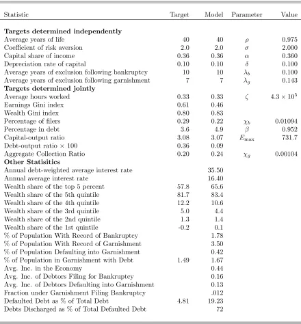
Table 1 gives the values of the parameters and the data targets that determine these parameters (for the
four parameters that are jointly determined, the assignment is to the data target that mostly determines
that parameter). Since we are calibrating to the wage process from the PSID, the earning inequality is not as
high as in the data. This discrepancy presumably reflects the fact that the PSID does not provide accurate
information on people with very high incomes. Although the PSID earnings process is augmented with the
super-rich and thus has a disproportionately strong effect on the capital output ratio.
18Domeij and Floden (2006) have noted that borrowing constraints could downwardly bias the estimate of labor supply
elasticity for certain specifications of utility functions. Our GHH specification does not suffer from this bias because labor supply is independent of consumption and therefore wealth.
19Lefgren and McIntyre (2009) (Table 2, pp. 376-77) report that 23 US states adhere to the federal guideline on the fraction
of disposable income that must be protected from garnishment (75 percent). Of the remaining states, 15 allow more than 75 percent to be protected from garnishment and the rest have an absolute minimum level of weekly earnings that are protected from garnishment.
20We thank Robert Hunt of the Federal Reserve Bank of Philadelphia’s Payment Cards Center for this estimate. Hunt reports
super-rich state, the fraction of people earning very high incomes is still very low so that the earnings Gini
is well below what is observed in the US data. But the addition of the super-rich state does help bring the
model Gini on wealth close to the data. The people who become super-rich have both the opportunity (very
high incomes) and the incentive (the state is very transitory) to accumulate large amounts of wealth. The
model is able to match the capital output ratio and the aggregate collections ratio fairly well but cannot
match the debt statistics exactly. The filing rate and the debt-to-output ratio are too low relative to the
data and the fraction of population in debt too high. To get more debt into the model, the interest rates on
debt must fall but that increases the fraction in debt further above target and tends to push the filing rate
further below target.21 The existing configuration is about the best the model can do. The average interest
rate paid by borrowers is 22 percent and the debt-weighted average is 35 percent.22
[Insert Table 1 here]
A novel feature of our model is the choice between bankruptcy and garnishment. In the bottom section of
Table 1 some statistics relevant to this choice are reported. In equilibrium, both options are active, with the
fraction defaulting and going into garnishment being 0.42 percent each period (as compared to 0.29 percent
for bankruptcy). The total stock of people with impaired credit (with either a bankruptcy or a garnishment
“flag” in their credit history) is 5.2 percent, with a majority having a garnishment flag.23 Although the
fraction filing for bankruptcy is only 34 percent of the total number of people defaulting, the fraction of debt
that is written off in bankruptcy is 72 percent of total defaulted debt. This is intuitive: Bankruptcy is not
the optimal choice when the individual wishes to default on a low level of debt because both the flow cost and
the duration of punishment is higher for bankruptcy than for garnishment. Consistent with this logic, the
average income of debtors filing under bankruptcy is higher than the average income of debtors defaulting
into garnishment (0.16 vs 0.13). Because the debt that goes into garnishment is relatively small, garnishment
generally does not last long: On average a person is under garnishment for 4 years. Most garnishments end
in full repayment of debt, with only 1.2 percent of debtors being garnished moving into bankruptcy each
period.24 The population in debt and being garnished is 1.67 percent. In the data, this number is between 1.5 and 1.7 percent, which is a remarkably good fit.25 Finally, the model predicts a much higher charge-off
rate than what is observed in the data. In the data, the average gross charge-off rate between 1984 and 2007
is 4.81 percent. The comparable statistic in the model is 19.23 percent. This deviation is to be expected
given the fact that we have too little debt in the model but the filing rate is about right.
21The difficulty in matching the debt-to-income ratio, the filing rate and percentage in debt seems to be common to this class
of models (see, for instance, Athreya, Tam and Young, 2009, and Chatterjee et al., 2007).
22These numbers seem high relative to reported interest rates. However, lenders often disguise interest charges as fees of
various sorts. For instance, if a borrower is paying 18 percent interest on a credit balance of $500 and is charged late fees of $35 twice, the effective annual interest rate is close to 32 percent.
23Since garnishment information appears in people’s credit history for some length of time, it should be possible to determine
what fraction of people are carrying a garnishment flag. Unfortunately, given the aggregated form in which credit bureau data are made available to researchers, it is not possible to determine this fraction.
24The probability of filing increases over time for people in garnishment: If a person under garnishment does not exit
garnishment, it is because his circumstances has either remained unchanged or deteriorated further. Further deterioration in earnings may trigger a bankruptcy filing.
25The figures are from PSID for 1997, 2002 and 2007. In these years, the survey asked (minor variations) of the following
Lefgren and McIntyre (2009) empirically examine the determinants of the frequency of Chapter 7 bankruptcy
filings across US states. Among other findings, they report that states that mandate a higher threshold and
protect a larger fraction of earnings above the threshold (restricted garnishment states) experience fewer
Chapter 7 filings (Table 3, p. 381). This prediction is against the model by confronting two small (more
precisely, measure zero) subsets of the model population with alternative garnishment laws: a less-restricted
garnishment law in whichcminis set to 0.1 times average earnings andγ= 0.25 (no state can haveγhigher
than 0.25) and a more-restricted law in whichcminis set to 0.61 times average earnings andγ= 0.10. The
long-run filing frequency is 0.25 for the less restricted garnishment law and 0.22 for the more restricted law.
Correspondingly, the frequency of garnishment is 0.13 in the former and 0.51 in the latter. Thus, filing
frequencies move in the direction consistent with the evidence, although the movement appears to be more
muted in the model than in the data.26
4
Eliminating Bankruptcy Protection
This section reports how prices, allocations and welfare are affected if bankruptcy protection (the right to
discharge of debt) is eliminated. Indebted households may still default but creditors have the right to collect
on their claims to the extent permitted by wage garnishment laws.
4.1
Allocations and Prices
Table 2 compares the baseline steady state with the garnishment-only steady state. In the garnishment
economy, all parameters that are common between the baseline and garnishment economies are set to the
values determined for the bankruptcy economy.
[Insert Table 2 here]
Comparison reveals some similarities and also some very striking differences. First, the average labor
supply in the two steady states are basically the same – actually, aggregate labor supply is slightly lower in
the garnishment economy. There are two reasons for this. First, labor supply is lower because wages are
lower (as we will see below). Second, garnishment distorts effort choices downward because of the “tax”
element. However, these effects do not amount to much because the elasticity of labor supply is low and an
individual will leave himself the possibility of being garnished only if it’s not that distortive for him (either
because the individual earns less thancminor he can pay off the debt quickly). Because labor supply is not
that much affected by the garnishment regime, the earnings Gini remains essentially the same.
The most striking difference between the two equilibria is in the debt measures. In the baseline economy
the percentage in debt is a little under 5 percent, but in the garnishment economy it is a little under 30
percent – an increase of a factor of 6. Additionally, the debt-to-output ratio goes from 0.09 percent to
around 22 percent. The proximate reason for this huge expansion in credit is a shift up ofq(a, s;p) schedule,
26This may be due to the fact that the model does not contain a third category of borrowers: the class of “informal bankrupts,”
stemming from a decline in the probability of default.27 The lower interest rates motivate people to borrow more and the expansion in debt continues until the default rate reaches roughly the same level as in the
baseline economy. Importantly, the elimination of discharge does not reduce the default – in fact, it increases
it.
Even though the default rate is only somewhat above the baseline economy, the fraction of people with
impaired credit (i.e., in bad standing) is much higher. The reason is that the duration of garnishment lasts
much longer now because when people default they do so on much larger levels of debt and it takes longer
to repay those debts and exit garnishment.
The increase in consumer credit can be expected to crowd out fixed capital, and it does, but surprisingly
little. The capital to output ratio declines from 3.08 to 2.97. The drop results in a slightly higher risk-free
interest rate, which rises from 1.74 percent to 2.05 percent, a rise of about 30 basis points. The decrease
in capital per worker results in a decline in wages of 1.67 percent. The decline in capital stock is muted
because of the presence of the super-rich. These individuals have a very elastic supply of savings and expand
their savings to accommodate the increased demand for consumer loans. If we eliminate the super-rich along
with discharge, the capital output ratio falls to 2.71 and the (net) rental return on capital climbs to 3.29
percent. Thus, getting the baseline wealth distribution to match reality (which necessitated the addition of
the super-rich state) has important implications for the counterfactual.
Finally, Table 2 shows that there is a massive increase in wealth inequality. This comes about because so
many individuals become indebted. The top 5 percent of the population ends up holding 66 percent of total
wealth in the garnishment-only economy compared with 56 percent in the baseline economy. The bottom
quintile has negative net-worth amounting to 7 percent of total wealth.
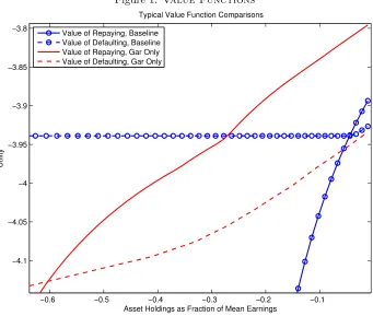
Why exactly does the incentive to default change so drastically in the garnishment economy? There are
two effects at work. One is the stick effect, which is that default is more costly to the individual, and the
other is the carrot effect, which is that maintaining access to markets is more beneficial. Figure 1 shows
that both effects are at work. The mostly flat dashed line with circles shows for a typical efficiency level
the value function of defaulting in the baseline economy, which is the maximum of declaring bankruptcy
and entering garnishment. The flat region is where bankruptcy is the best option. The dashed line without
circles is the value of defaulting in the garnishment-only economy. Observe that as the debt level rises,
default in the garnishment-only economy becomes increasingly worse relative to the value of default in the
baseline. This is the stick effect of garnishment: default under garnishment is simply not as beneficial to
the individual as default under bankruptcy. The solid line with and the solid line without circles show the
value function conditional on repaying debt in the baseline and garnishment-only economies respectively.
Notice that the value of repaying debt in the garnishment-only economy lies considerably above the value of
repaying debt in the baseline. This is the carrot effect of garnishment: by lowering the costs of borrowing, the
garnishment-only economy increases the value of maintaining access to the credit market. The lens-shaped
areas trapped between the solid and dashed lines is where households do not default. This area is much
larger in the garnishment-only economy because of these two effects.
27Athreya (2008, Table 1 p. 762) reports what happens ifdefaultis eliminated, so individuals can borrow at the risk-free rate
[Insert Figure 1 here]
The increased value of maintaining access to the credit market is apparent in the positioning of the
price schedules in the baseline and the garnishment-only economies. Figure 2 shows the average loan price
for the two economies for different levels of debt: credit is available under more generous terms in the
garnishment-only economy than in the baseline economy. Competitive lenders are willing to extend loans
on more generous terms because debtors do not default as much, and even when they do default, they pay
their debts back in due course.
[Insert Figure 2 here]
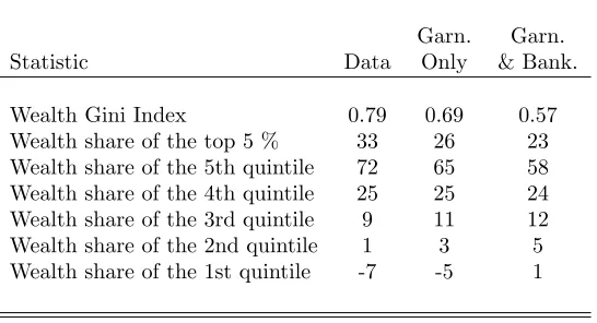
Is the large increase in wealth inequality a credible implication of the lack of discharge? A case in point
is Sweden, which until 2005 did not permit discharge of debt and, yet, Sweden does not have the wealth
inequality predicted by our model. But Sweden’s income process is different as well. Table 3 reports wealth
distribution statistics if the US garnishment-only economy is fed Sweden’s income process, also estimated
and presented in Floden and Linde (2001).28 All other parameters are exactly as in the US economy, except forξ, which is set to a value for which the highest paid person in Sweden works twice as long as the lowest
paid person. The table also reports the wealth distribution statistics for Sweden taken from Domeij and
Klein (1998). As is evident, the wealth distribution for our “Swedish” economy is surprisingly close to the
actual Swedish wealth distribution. In particular, the bottom 20 percent of the population, on aggregate,
hold debt (as opposed to assets) in both the model economy as well as in the data. Indeed, the level of
indebtedness in the Swedish data is actually higher than in our “Swedish” model.29 This limited exercise
indicates that the “extreme” distributional implications of the US garnishment-only economy may reflect
the much greater degree of income risk in the US compared to European economies. Also, if Sweden were
to adopt US style discharge laws, then, as shown in the final column, the bottom quintile will become net
savers; the capital output ratio will rise; and the distribution of wealth would look less unequal.
[Insert Table 3 here]
4.2
Welfare
The welfare effects of eliminating bankruptcy protection are now presented. The first measure gives the flow
consumption a person would give up to go from a regime in which there is bankruptcy to a regime in which
bankruptcy is eliminated.30 The second measure simply counts the fraction of people who would be in favor
of eliminating bankruptcy. The latter measure provides insight into the degree of political support in favor
of or against the institution of bankruptcy.
In both cases, it is assumed that the question is posed in an unanticipated mannerafter people have made
their default decision but before they have chosen their new asset positions. This timing ensures that the
contemplated switch in regime does not impose unanticipated profits or losses on the intermediary sector.31
28The AR1 coefficient on the persistent process is 0.8139 and the variance of the innovation to this process is 0.0326; the
variance of the permanent shock is 0.0467 and the variance of the transitory shock is .0251.
29We should note that there are competing explanations for the large fraction of negative networth individuals in Sweden.
Domeij and Klein (2002) argue that it is the nature of the Swedish public pension system that accounts for Sweden’s considerable wealth inequality despite Sweden having a relatively low earnings inequality.
30The consumption equivalent measure is computed as follows: Given policiesc(a, e, h), n(a, e, h),andd(a, e, h) corresponding
to a value functionV(a, e, h), the value of using policies ˜c(a, e, h) = (1 + Γ)c(a, e, h)n(a, e, h),andd(a, e, h) forever is computed using policy iteration. This is done for 30 values of Γ between -.9 and 2. To find the Γ for which ˜V(a, e, h; Γ) equals some level of utilityW, a nonlinear equation solver (interpolating ˜V in the Γ dimension) is used.
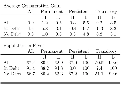
The top panel of Table 4 reports the consumption equivalent measure from eliminating bankruptcy,
taking into account the transition to the new steady state. Each cell gives the consumption flow averaged
across the cell’s households. Overall, there is a significant gain from eliminating bankruptcy – amounting
to about 1.0 percent of consumption in perpetuity. The gain is not uniform: Indebted people gain more
than others. This makes sense because borrowing is cheaper in the garnishment-only economy. The income
level matters as well: those receiving the lowest persistent or transitory efficiency shocks gain the most and
those receiving the highest shocks the least. This pattern reflects the fact that those in need of loans are the
ones who gain most from the decrease in borrowing rates. For the permanent shock, the pattern of relative
gain is reversed: those with the highest permanent shock gain more than those with the lowest permanent
shock. The high permanent shock individuals own a large amount of assets and they prefer the garnishment
because of the higher associated interest rate on savings.
[Insert Table 4 here]
The bottom panel of the table reports the fraction of people in each cell in favor of eliminating bankruptcy
protection. About 10 percent of the population opposes it and, interestingly, they are drawn mostly from the
ranks of indebted people with high persistent and transitory efficiency shocks. Why do these people oppose
the elimination of discharge? Because they have high income which mean revert, their need to borrow is
low and because they are indebted, they are unlikely to have a high level of assets. For these individuals
the main effect on welfare comes from the decline in real wages. The effect is small (because the decline in
wages in small) but they oppose the change, nevertheless.
Although factor prices do not change very much from one steady state to the other, Table 5 indicates that
the steady state welfare gains are about 0.2 percentage point, or less, lower than those taking the transition
into account. Also, ignoring the transition can give a misleading picture of the degree of political support
for the elimination of bankruptcy. Without the added benefit of the higher consumption afforded by the
de-accumulation of capital, support for elimination of discharge is much lower. Overall, only 67 percent of
the population now favors eliminating discharge.
[Insert Table 5 here]
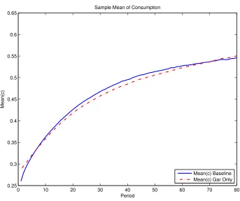
Garnishment increases the value of maintaining access to credit markets and allows for an expansion of
credit. It is useful to understand exactly what this expansion allows in terms of consumption profiles. With
this in mind, a large number of individuals were simulated who “start life” witha= 0,h= 0 ande drawn
from the invariant distribution. Their consumption and asset holdings were recorded for the next 80 periods
(years) under both the bankruptcy steady state and the garnishment steady state. The following two figures
display average consumption and average asset holdings across the two regimes for each of the 80 periods.
Figure 3 shows that mean asset holdings rise more slowly in the garnishment-only economy, whereas
they increase rapidly in the bankruptcy economy. In the latter, the high cost of loans forces individuals to
accumulate assets in order to self-insure. In the garnishment economy, the need to accumulate precautionary
savings is much less urgent, since the loan supply schedule is much more attractive. Mean consumption is
higher in the garnishment economy because people are saving less. Mean consumption is higher for some
time until the accumulated debt burden begins to lower consumption below that in the baseline economy.
[Insert Figure 3 here]
The effects of better consumption smoothing can be seen in Figure 4 which displays the coefficient of
variation of consumption for each age. Observe that the coefficient of variation is initially lower in the
garnishment-only economy but then exceeds that of the baseline economy. It is lower initially because of
the superior consumption smoothing afforded by the generous loan supply schedules in the garnishment-only
economy. But the other side of the same coin is the increased dispersion of asset holdings resulting from
enhanced borrowing and lending. Higher wealth inequality eventually translates into higher consumption
inequality.
[Insert Figure 4 here]
Finally, the optimal garnishment regime, if discharge were to be eliminated, is investigated. This exercise
is motivated by the consideration that elimination of discharge is a large institutional change that, if it were
to be instituted, would almost surely result in significant changes in garnishment law as well. The average
steady-state consumption gains for a range ofcminandγ values wer computed.32 The optimal garnishment
regime is one with γ = 1 and cmin = 0. This is a “zero tolerance for delinquency” regime in which the
creditors have the right to garnishall of the debtor’s earnings in case of default. Eliminating discharge and
instituting this garnishment regime raises average steady state welfare by 3.71 percent as compared to 0.856
percent for the current garnishment regime. The optimal garnishment economy is essentially a “natural
borrowing limit” (a la Aiyagari, 1994) economy with no default. There is novoluntary default because the
creditors can garnish earnings fully to recover the defaulted debt so the defaulter does not gain current
consumption but pays the reputation costs associated with a bad credit history. And there is noinvoluntary
default because individuals never find it in their interest to borrow more than the amount that can be rolled
over even in the event the debtor has the lowest efficiency level. For the baseline calibration, this natural
borrowing limit is −1.58, or roughly 360 percent larger than average income in the economy. In contrast,
the maximum amount that an individual would wish to borrow in the current garnishment regime (with no
discharge) is−0.93, or roughly 210 percent larger than average income in the economy.33
This logic makes clear that the optimality of the “zero tolerance” regime hinges on the size of the lowest
efficiency level.34 If this level is very low – “a disaster state” – the optimal garnishment economy will not
be the “zero tolerance” one. This point is verified by augmenting the income process with an efficiency
level that corresponds to a super-poor state, which happens with a very small probability and is very
transitory.35 Addition of this state does not change model statistics in the baseline economy because the
probability of the super-poor state is very low and the individual debtor always has the option to declare
bankruptcy.36 However, once bankruptcy protection is eliminated, the event looms large in the utility
calculation of individuals. Basically, the presence of this state raises the welfare gain from elimination of
discharge for low punishment regimes and lowers it for high punishment regimes. For instance, the welfare
gain for the current regime rises from 0.841 percent to 0.917 percent and that for the “zero tolerance” regime
32We ignored the transition because it is time consuming to compute.
33The most that a lender would wish to borrow is the debt level at whichq(a0, s)a0 is maximized. Although the individual can borrow more than this, he would not want to because the borrower gets less in terms of current consumption and is saddled with more debt in the future.
34In the discretized income process of the baseline economy, the minimum efficiency level is a positive number although the
true distribution allows for efficiency levels arbitrarily close to zero with vanishingly small probability.
35The efficiency level is 5 standard deviations below the unconditional mean of the log-efficiency process. It is iid and occurs
with probability 1 in 3.5 million (which is the mass 5 standard deviations or more below the mean of a normal distribution).
36For example, both the population in debt and the population filing for bankruptcy are unchanged. The capital-output ratio
declines from 3.710 percent to 2.076 percent. Furthermore, the “zero tolerance ” regime is no longer optimal;
the optimal regime now hasγ= 0.50 andcmin= 0. These results are indicative of the welfare results would
change if wealth/liability shocks had been included in the model. As noted in Chatterjee et al. (2007) and
in Livshits et al. (2007), wealth shocks stemming from uninsured medical expenses are an important trigger
for bankruptcy. Including such shocks will likely reduce the welfare gain from elimination of discharge. In
this sense, our welfare estimates should be viewed as an upper bound.
5
Conclusion
The concluding section attempts to put the findings of this project into perspective and draws some lessons
regarding what might be useful research lines to pursue in the general area of consumer default.
A question one might ask is whether the findings reported in this paperfirmlysupport the notion that the
US economy would be better off without bankruptcy protection? Although a 1 percent increase in welfare is
large by the standards of macroeconomic analysis, this gain must be set against costs ignored in this study.
One cost that has been ignored is the cost of enforcing garnishment laws. In the baseline economy, less than
2 percent of the population suffer garnishment each period; in the counterfactual, close to 16 percent do. To
process such a large volume of garnishments the administrative and legal resources devoted to this task must
be increased very substantially. Second, a society with as extreme a wealth distribution as the
garnishment-only economy would presumably suffer from political and social costs. These missing costs suggest that the
findings reported in this paper do not provide a convincing case for elimination of bankruptcy protection, at
least given current garnishment laws.
This, then, raises the question whether default policy should move in the direction of eliminating
bankruptcy protection and toughening up garnishment laws. A strong commitment to honor one’s debt
works well if it is combined with forward-looking behavior that steers individuals away from truly bad
finan-cial situations. But the train of events of the last several years shows that individuals may not possess the
requisite foresight to pull this off. After decades of low aggregate volatility, the Great Contraction caught
people and policymakers by surprise. The design of legal institutions that can facilitate the optimal societal
response to unexpected situations remains an open and important task. In this quest, historical experience
can serve as a guide: In the pre-discharge era, state legislatures granted delinquent debtors one-time debt
forgiveness when macroeconomic conditions were particularly bad. Estimating the net benefits of tough
garnishment laws coupled with state-contingent bankruptcy protection would seem to be a useful line of
research.
Another question one might ask is what lessons do quantitative-theoretic models offer for conventional
empirical research on consumer default? Empirical studies (well-known examples are Fay, Hurst and White
(2002) and Gross and Souleles (2002)) focus on testing the sign restrictions on regression coefficients implied
by simple models of default. Quantitative-theoretic models go beyond simple default models in making
predictions regarding themagnitude of the various effects as well. This added quantitative information can
be useful in interpreting empirical findings, in terms of the importance of the various causal mechanisms
at work. A case in point is the muted effect of variation in garnishment restrictions (all else remaining the
same) on bankruptcy filing rates in the model. As noted earlier, this difference may arise from the presence
in Chapter 7 homestead exemptions. Furthermore, the fact that quantitative-theoretic models are fully
articulated artificial economies composed of heterogeneous agents operating through time can be leveraged
to generate artificial data of the type available to empirical researchers and which can then be approached
in same way researchers approach real data. This procedure can illuminate the strengths and weaknesses of
empirical specifications in uncovering causal links that researchers believe exist in reality – and which exist
for sure in the model-generated data – but can get distorted, or masked, by data limitations (Chen, 2010).
Aside from enriching the interplay between theory and empirics, quantitative-theoretic models may alert
empirical researchers to regularities that should exist in the data, if the underlying theory is correct. One
example of this is the prediction that the costs of garnishment ought to be lower than costs of bankruptcy and
that debts collected in garnishment should be smaller, on average, than debts written-off in bankruptcy. The
feedback can also go the other way: Fay, Hurst and White’s finding that many individuals forego bankruptcy
even when it is financially beneficial have motivated quantitative theorists to include heterogeneous
non-pecuniary costs of bankruptcy filings (Athreya, Tam and Young, 2009).
References
Aiyagari, S., 1994. Uninsured idiosyncratic risk and aggregate savings. Quarterly Journal of Economics
109 (3), 659–684.
Athreya, K., 2002. Welfare implications of the bankruptcy reform act of 1999. Journal of Monetary Economics
49 (8), 1567–1595.
Athreya, K., 2008. Default, insurance and debt over the life-cycle. Journal of Monetary Economics 55 (4),
752–774.
Athreya, K. B., Tam, X. S., Young, E. R., 2009. Are harsh penalties for default really better? Working
Paper 09-11, Federal Reserve Bank of Richmond.
Chatterjee, S., Corbae, D., Nakajima, M., R´ıos-Rull, J.-V., 2007. A quantitative theory of unsecured
con-sumer credit with risk of default. Econometrica 75 (6), 1525–1589.
Chatterjee, S., Corbae, D., R´ıos-Rull, J.-V., 2011. A theory of credit scoring and the competitive pricing of
default risk, mimeo.
Chatterjee, S., Eyigungor, B., 2010. Maturity, indebtedness and default risk. Working Paper 10-12, Federal
Reserve Bank of Philadelphia.
Chen, D., 2010. Impact of personal bankruptcy on labor supply decisions, mimeo.
Coleman, P. J., 1999. Debtors and Creditors in America: Insolvency, Imprisonment for Debt, and
Bankruptcy, 1607-1900. BeardBooks, Washington D.C.
Dawsey, A., Ausubel, M., 2004. Informal bankruptcy, mimeo.
Dawsey, A., Hynes, R., Ausubel, M., 2004. The regulation of non-judicial debt collection and the consumer’s
Domeij, D., Floden, M., 2006. The labor supply elasticity and borrowing constraints: Why estimates are
biased. Review of Economic Dynamics 9 (2), 242–262.
Domeij, D., Klein, P., 1998. Inequality of wealth and income in Sweden, mimeo.
Domeij, D., Klein, P., 2002. Public pensions: To what extent do they account for Swedish wealth inequality?
Review of Economic Dynamics 5 (3), 503–534.
Edelberg, W., 2006. Risk-based pricing of interest rates for consumer loans. Journal of Monetary Economics
53 (8), 2283–2298.
Fay, S., Hurst, E., White, M., 2002. The household bankruptcy decision. American Economic Review 92 (3),
706–718.
Floden, M., Linde, J., 2001. Idiosyncratic risk in the US and Sweden: Is there a role for government insurance?
Review of Economic Dynamics 4 (2), 406–437.
Greenwood, J., Hercowitz, Z., Huffman, G. W., 1988. Investment, capacity utilization, and the real business
cycle. American Economic Review 78 (3), 402–417.
Gross, D., Souleles, N., 2002. An empirical analysis of personal bankruptcy and delinquency. Review of
Financial Studies 15 (1), 319–347.
Lefgren, L., McIntyre, F., 2009. Explaining the puzzle of cross-state differences in bankruptcy rates. Journal
of Law and Economics 52 (2), 367–393.
Li, W., Han, S., 2007. Fresh start or head start? the effects of filing for personal bankruptcy on work effort.
Journal of Financial Services Research 31 (2), 123–152.
Li, W., Sarte, P., 2006. U.S. consumer bankruptcy choice: The importance of general equilibrium effects.
Journal of Monetary Economics 53 (3), 613–631.
Li, W., White, M., 2009. Mortgage default, foreclosure and bankruptcy. Working Paper 15472, NBER.
Livshits, I., MacGee, J., Tertilt, M., 2003. Consumer bankruptcy: a fresh start. Working Paper 617, Federal
Reserve Bank of Minneapolis.
Livshits, I., MacGee, J., Tertilt, M., 2007. Consumer bankruptcy: a fresh start. American Economic Review
97 (1), 402–418.
Mehlkopf, R., 2010. Intergenerational risk sharing under endogenous labor supply, mimeo.
Mitman, K., 2011. Macroeconomic effects of bankruptcy and foreclosure policies. PIER Working Paper
11-015, University of Pennsylvania.
Musto, D., 2004. What happens when information leaves a market? evidence from post-bankruptcy
con-sumers. Journal of Business 77 (4), 725–748.
Table 1: Model Statistics and Parameter Values
Statistic Target Model Parameter Value
Targets determined independently
Average years of life 40 40 ρ 0.975
Coefficient of risk aversion 2.0 2.0 σ 2.000
Capital share of income 0.36 0.36 α 0.360
Depreciation rate of capital 0.10 0.10 δ 0.100
Average years of exclusion following bankruptcy 10 10 λb 0.100
Average years of exclusion following garnishment 7 7 λg 0.143
Targets determined jointly
Average hours worked 0.33 0.33 ζ 4.3×10⁵
Earnings Gini index 0.61 0.46
Wealth Gini index 0.80 0.83
Percentage of filers 0.29 0.22 χb 0.01094
Percentage in debt 3.6 4.9 β 0.952
Capital-output ratio 3.08 3.07 Emax 731.7
Debt-output ratio×100 0.36 0.09
Aggregate Collection Ratio 0.20 0.24 χg 0.00104
Other Statisitics
Annual debt-weighted average interest rate 35.50
Annual average interest rate 16.40
Wealth share of the top 5 percent 57.8 65.6
Wealth share of the 5th quintile 81.7 83.4
Wealth share of the 4th quintile 12.2 10.6
Wealth share of the 3rd quintile 5.0 4.4
Wealth share of the 2nd quintile 1.3 1.4
Wealth share of the 1st quintile -0.2 0.1
% of Population With Record of Bankruptcy 1.78
% of Population With Record of Garnishment 3.50 % of Population Defaulting into Garnishment 0.42 % of Population in Garnishment with Debt 1.49 1.67
Avg. Inc. in the Economy 0.44
Avg. Inc. of Debtors Filing for Bankruptcy 0.16 Avg. Inc. of Debtors Defaulting into Garnishment 0.13 Fraction under Garnishment Filing Bankruptcy .012
Defaulted Debt as % of Total Debt 4.81 19.23
Debts Discharged as % of Total Defaulted Debt 72
Note: The table lists some US statistics with the corresponding statistics in the model, as well as the
parameter values that most closely affect the model statistics. Where the US statistic is not known, its value
is left blank. The parameters are as follows: ρ is a conditional probability of survival, σ is the coefficient
of relative risk aversion, αis the capital share of income, δ is the depreciation rate of capital, λb and λg
are the probabilities that a record of bankruptcy respectively garnishment is removed from an individual’s
disutility cost of labor,β is the time discount factor, andEmax is the efficiency of the super-rich households