P-Waves Interaction with Crack at Orthotropic Interface

P-waves interaction with crack at orthotropic

interface

Palas Mandal∗, Subhas Chandra Mandal†

Department of Mathematics, Jadavpur University, Kolkata-700032, West Bengal, India.

Abstract: The paper is concerned with the problem of diffraction of P-waves by a Griffith crack situated at the interface of two different orthotropic media has been analyzed. Using Fourier transform and integral equation method, the mixed boundary value problem has been reduced to the solution of dual integral equations which has finally been reduced to the solution of a Fredholm integral equation of the second kind which are finally solved by using perturbation method. Stress intensity factor(SIF) and crack opening displacement (COD) around the crack tip are derived. The values of SIF and crack opening displacement have been calculated for various type of orthotropic materials and depicted graphically.

Key Words: Griffith crack, Orthotropic media, P-wave, Stress intensity factor, Crack opening displacement.

I. Introduction

In recent years the problems of diffraction of elastic waves by cracks are of considerable importance in view of their application in Engineering Mathematics. The primary objective in engineering structure is to avoid the growth of the crack once it initiated. It was found that the stress has a square root singularity at the tip of the crack. In this prospect a non-dimensional quantity called stress intensity factor is used to predict the stress state near the crack tip caused by an applied load. Many researchers did their work on wave propagation on bonded media containing an interfacial crack. Fracture mechanics and study of crack propagation can be considered as an interesting branch in elastic theory. The performance of engineered systems is affected by inhomogeneities such as cracks and inclusions present in the material. Theory and problems related to crack geometry in orthotropic materials have emerged as a very interesting area of research in recent times mostly due to the rapid growth in construction engineering. Anisotropy and flaw at the interface of two bonded materials are of great importance in designing engineering structures and machines. Composite materials are becoming an essential commodity in modern era as they offer advantages such as low weight to strength ratio, corrosion resistance, and high fatigue strength. The growing use of composite materials in many engineering applications demand the fundamental understanding of the response of cracked orthotropic bodies under stress. Many composite materials are used in making aircraft structures to golf clubs, electronic packaging to medical equipment, and space

vehicles to home building. It has been observed that applications of composite materials in the commercial market are also increasing day by day. The crack problem in fracture mechanics has a wide range of applications in civil engineering. It has a big application on manufacturing engineering for designing metal and polymer forming processes, machining, etc.

Srivastava et al. [22] solved the problem of interaction of shear waves with Griffith crack situated at the interface of two bonded dissimilar elastic half spaces. The problem becomes more difficult and complicated when boundaries are present in the media. Li [14] obtained the analytical solution for a static problem of two bonded orthotropic strips containing an interfacial crack. The dynamical problem was studied by Matbuly [18] and obtained the analytical expression of stress intensity factor. Diffraction problems involving multiple cracks had been studied by many authors. But most of the problems were either involving diffraction of shear waves or diffraction in infinite media. E. Lira-Vergara and C. Rubio-Gonzalez

[12-13] obtained the dynamic stress intensity factor of interfacial finite cracks in orthotropic

materials. Itou [7] considered the diffraction problem of an antiplane shear wave by two coplanar Griffith cracks in an infinite elastic medium. Stress distribution near periodic cracks at the interface of two bonded dissimilar orthotropic half planes was studied by Garg [6]. The problem of diffraction of elastic waves by two coplanar Griffith cracks in an infinite elastic medium was solved by Jain and Kanwal [10]. The transient response of two cracks at the interface of a layered half space had been investigated by Kundu [11]. Mandal and Ghosh [15] solved the problem of interaction of elastic waves with a periodic array of coplanar Griffith cracks in an orthotropic medium. Diffraction problem of three coplanar Griffith cracks in an orthotropic medium was considered by Sarkar et al. [20]. Das [3] and others considered the problems containing a Griffith crack in an transversly orthotropic medium. Mukherjee et al. [17] have studied the interaction of three interfacial Griffith cracks between bonded dissimilar orthotropic half planes and find out the stress intensity factor. Satapathy et al. [19] considered an orthotropic strip containing a Griffith crack which is finally solved. Daset al. [4]are finding the Stress intensity factor of an edge crack in bonded orthotropic materials. Dynamic stress intensity factors of multiple cracks in an orthotropic strip with FGM coating was studied by Monfared and Ayatollahi [16]. Sinharoy [21] solved elastostatic problem of an infinite row of parallel cracks in an orthotropic medium under general loading. Itou [9] solved the problem of dynamic stress intensity factors of three collinear cracks in an orthotropic plate subjected to time-harmonic disturbance

In most of the above discussed papers, the problem involving the P-waves on a finite crack with two semi-infinite elastic half-spaces. Therefore we state the problem as diffraction of P-waves in two bonded dissimilar containing a Griffith crack at the interface. The Fourier transform is used to reduce the problem to a system of dual integral equations . Then the set of dual integral equation is further reduced to a Fredholm integral equation of second kind by using Abel’s transform technique. The solution of this integral equation has been obtained for low frequency by using perturbation method. An iterative procedure is adopted to obtain the low frequency solution of the problem. This procedure leads to obtain the analytical expressions of the stress intensity factor (SIF) and crack opening displacement. Finally the effect of material constants, on stress intensity factor and crack opening displacement have been shown by virtue of the graphs.

II. Formulation of the problem

consider the transformationx1/a=x,y1/a=y andz1/a=z, then we find that the location

of the crack at the interface becomes|x|<1,−∞< z <∞,y= 0.

-

1

1

_x

y

z

Medium 1

Medium 2

Fig.1 Configuration of the Crack

The displacementsux(x, y) anduy(x, y) along thexand y axes respectively are given by the

following equations

c(₁₁k)∂ 2_u(k)

x

∂x2 + ∂2u(xk)

∂y2 + (1 +c (k) 12)

∂2u(yk)

∂x∂y = a2 c2

s

∂2u(xk)

∂t2 , k= 1,2. (1)

c(₁₁k)∂ 2_u(k)

y

∂x2 + ∂2u(yk)

∂y2 + (1 +c (k) 12)

∂2u(xk)

∂x∂y = a2 c2

s

∂2u(yk)

∂t2 , k= 1,2. (2)

wherec11, c22and c12are non-dimensional parameters related to the elastic constants by the

relations

c11= E1

µ12[1−( E₂ E1)µ

2 12]

c22= E_E2₁c11

c12=ν12c22=ν21c11

In the above equations Ei, µij and νij (i, j = 1, 2, 3) denote the engineering elastic

constants of the material where the subscript 1, 2, 3 correspond to the x, y, z directions which coincide with the axis of material orthotropy and the constantsEi andνij satisfy the

Maxwell’s relation νij/Ei = νji/Ej. Therefore, substituting ux(x, y, t) = ux(x, y)e−iωt and

uy(x, y, t) =uy(x, y)e−iωt in equations (1) and (2) we obtain

c(₁₁k)∂ 2_u(k)

x

∂x2 + ∂2u(xk)

∂y2 + (1 +c (k) 12)

∂2u(yk)

∂x∂y +k 2

c(₁₁k)∂ 2_u(k)

y

∂x2 + ∂2u(yk)

∂y2 + (1 +c (k) 12)

∂2u(xk)

∂x∂y +k 2

su(yk)= 0, k= 1,2. (4)

The stresses and displacements are related by the following equations

σyy(k)/µ₁₂(k)=c(₁₂k)∂u (k) x ∂x +c

(k) 22

∂u(yk) ∂y

σxy(k)/µ(₁₂k)= ∂u (k) x ∂y +

∂u(yk) ∂x

σxx(k)/µ₁₂(k)=c(₁₁k)∂u (k) x ∂x +c

(k) 12

∂u(yk) ∂y

Henceforth the time factore−iωt which is common to all field variables would be omitted in the sequence but to be understood.

The boundary conditions are given by

σ_yy(1)(x,0+) =σ_yy(2)(x,0−) =−σ0, |x|<1 (5)

u(1)_y (x,0+) =u(2)_y (x,0−), |x|>1 (6)

u(1)_x (x,0+) =u(2)_x (x,0−), |x|>1 (7)

σ_yy(1)(x,0+) =σ_yy(2)(x,0−), |x|>1 (8)

σ(1)_xy(x,0+) =σ(2)_xy(x,0−), |x|<∞ (9)

The displacement component ux in x direction is negligible in comparison to the

displacement component uy in y direction in the case of normally incidence. We consider

that the displacement on the crack facesux(x,0+) anduy(x,0−) are identical. So for that in

lieu of (7) we consider

u(1)x (x,0+) =u(2)x (x,0−) for|x|<∞. (7a)

An appropriate integral solutions of (3) and (4) can be taken as

u(1)_x (x, y) = 2

π ∫ _∞

0

[A1(ζ)e−δ1y+A2(ζ)e−δ2y] sin(ζx)dζ y >0 (10)

u(2)_x (x, y) = 2

π ∫ _∞

0

[A′₁(ζ)eδ1y_+A′

2(ζ)eδ2y] sin(ζx)dζ y <0 (11)

u(1)_y (x, y) = 2

π ∫ _∞

0

1

ζ[ω1A1(ζ)e

−δ1y_+ω

2A2(ζ)e−δ2y] cos(ζx)dζ y >0 (12)

u(2)_y (x, y) = 2

π ∫ _∞

0

1

ζ[ω1A

′

1(ζ)eδ1y+ω2A

′

and the non vanishing stress components are given by

σ_xy(1)(x, y) =µ(1)₁₂ [

2

π ∫ _∞

0

{−A1(ζ)δ1e−δ1y−A2(ζ)δ2e−δ2y}sin(ζx)dζ

−2 π

∫ _∞

0

{ω1A1(ζ)e−δ1y+ω2A2(ζ)e−δ2y}sin(ζx)dζ ]

(14)

σ(2)_xy(x, y) =µ(2)₁₂ [

2

π ∫ _∞

0

{A′₁(ζ)δ1eδ1y+A

′

2(ζ)δ2eδ2y}sin(ζx)dζ

−2 π

∫ _∞

0

{ω1A

′

1(ζ)eδ1y+ω2A

′

2(ζ)eδ2y}sin(ζx)dζ ]

(15)

σ(1)_yy(x, y) =µ(1)₁₂ [

2c(1)₁₂ π

∫ _∞

0

{A1(ζ)e−δ1y+A2(ζ)e−δ2y}ζcos(ζx)dζ

+2c

(1) 22 π ∫ _∞ 0 1

ζ{−ω1A1(ζ)e

−δ1y_δ

1−ω2A2(ζ)e−δ2yδ2}cos(ζx)dζ ]

(16)

σ(2)_yy(x, y) =µ(2)₁₂ [

2c(2)₁₂ π

∫ _∞

0

{A′₁(ζ)eδ1y_+A′

2(ζ)eδ2y}ζcos(ζx)dζ

−2c (2) 22 π ∫ _∞ 0 1

ζ{ω1A

′

1(ζ)eδ1yδ1+ω2A

′

2(ζ)eδ2yδ2}cos(ζx)dζ ]

(17)

where

ωi =

c(₁₁k)ζ2_−k2 s−δi2

δi(1+c(₁₂k)) i= 1,2

and Ai(ζ)(i= 1,2), A

′

i(ζ)(i= 1,2) are the unknown functions to be determined, δ21 and δ22

are the roots of the equation

c(₂₂k)δ4+{((c(₁₂k))2+ 2c₁₂(k)−c₁₁(k)c(₂₂k))ζ2+ (1 +c(₂₂k))k_s2}δ2+ (c₁₁(k)ζ2−k_s2)(ζ2−k2_s) = 0 (18)

III. Derivation of the integral equation

From the boundary conditionsσ(1)yy(x,0+)−σyy(2)(x,0−) = 0 andσxy(1)(x,0+)−σxy(2)(x,0−) = 0

we obtain the relations between A2, A′1, A′2 and A1, A′1, A′2 as

A2 =A′1T11+A′2Q11 (19)

A1 =A′1R11+A′2S11 (20)

where

T11=

(µ(2)₁₂c(2)₁₂ζ+µ(2)₁₂c(2)₂₂ω1δ1 ζ ) + (µ

(1) 12c

(1) 12ζ+µ

(1) 12c

(1) 22

ω1δ1 ζ )

(δ1µ(2)12−ω1µ(2)12)

(δ1µ(2)12−ω1µ(2)12) (µ(1)₁₂c(1)₁₂ζ+µ(1)₁₂c(1)₂₂ ω1δ1

ζ ) + (µ

(1) 12c

(1) 12ζ+µ

(1) 12c

(1) 22

ω1δ1 ζ )

(δ2+ω2)

Q11=

(µ(2)₁₂c(2)₁₂ζ+µ(2)₁₂c(2)₂₂ ω2δ2 ζ ) + (µ

(1) 12c

(1) 12ζ+µ

(1) 12c

(1) 22

ω1δ1 ζ )

(δ2µ(2)12−ω2µ(2)12)

(δ1µ(2)12−ω1µ(2)12) (µ(1)₁₂c(1)₁₂ζ+µ(1)₁₂c(1)₂₂ ω1δ1

ζ ) + (µ

(1) 12c

(1) 12ζ+µ

(1) 12c

(1) 22

ω1δ1 ζ )

(δ2+ω2)

(δ1+ω1)

R11=−

δ2µ(1)₁₂ +ω2µ(1)₁₂

δ1µ(1)₁₂ +ω1µ(1)₁₂ .

(µ(2)₁₂c(2)₁₂ζ+µ(2)₁₂c(2)₂₂ ω1δ1 ζ ) + (µ

(1) 12c

(1) 12ζ+µ

(1) 12c

(1) 22

ω1δ1 ζ )

(δ1µ(2)12−ω1µ(2)12)

(δ1µ(2)12−ω1µ(2)12) (µ(1)₁₂c(1)₁₂ζ+µ(1)₁₂c(1)₂₂ ω1δ1

ζ ) + (µ

(1) 12c

(1) 12ζ+µ

(1) 12c

(1) 22

ω1δ1 ζ )

(δ2+ω2)

(δ1+ω1)

−δ1µ(2)12 −ω1µ(2)12 δ1µ(1)12 +ω1µ(1)12

S11=−

δ2µ(1)₁₂ +ω2µ(1)₁₂

δ1µ(1)12 +ω1µ(1)12 .

(µ(2)₁₂c(2)₁₂ζ+µ(2)₁₂c(2)₂₂ω2δ2 ζ ) + (µ

(1) 12c

(1) 12ζ+µ

(1) 12c

(1) 22 ω1ζδ1)

(δ2µ(2)12−ω2µ(2)12)

(δ1µ(2)₁₂−ω1µ(2)₁₂) (µ(1)₁₂c(1)₁₂ζ+µ(1)₁₂c(1)₂₂ ω1δ1

ζ ) + (µ

(1) 12c

(1) 12ζ+µ

(1) 12c

(1) 22ω1ζδ1)

(δ2+ω2)

(δ1+ω1)

−δ2µ(2)12 −ω2µ(2)12 δ1µ(1)₁₂ +ω1µ(1)₁₂

Applying the boundary condition (7a) and using the equations (19) and (20) in (10) and (11) we obtain the relation betweenA′₁ andA′₂ as

A′₂ =−βA′₁ (21)

where β = T11+R11−1 S11+Q11−1

The boundary conditions (5) and (6) lead to the following dual integral equations

∫ _∞

0

G(ζ)D(ζ) cos(ζx)dζ=− σ0 2µ(1)₁₂

, |x|<1 (22)

∫ _∞

0

D(ζ) cos(ζx)dζ= 0 |x|>1 (23)

where

G(ζ) = 1

(ω1R11+ω2T11−ω1S11β−ω2Q11β−ω1+ω2β) [

c(1)₁₂ π (ζ

2_R 11+

ζ2T11−βζ2Q11)− c(1)₂₂

π (ω1δ1R11+ω2δ2T11−ω1δ1βS11−ω2δ2Q11β) ]

(24)

and

D(ζ) =

[

ω1R11+ω2T11−ω1S11β−ω2Q11β−ω1+ω2β ]

A′₁(ζ)

ζ (25)

We consider

D(ζ) = 1

ζ ∫ 1

0

h(t) sin(ζt)dt (26)

to obtain the solution of integral equation (22) and (23) in whichh(t) is the unknown function which has been determined from the boundary conditions. Now using (26) in (22), we have obtained

d dx

∫ 1

0

h(t)dt ∫ _∞

0

ζsin(ζt) sin(ζx)G(ζ)

ζ dξ=−

σ0

2µ(1)₁₂

, 0< x <1 (27)

Using the relations

∫ _∞

0

sin(ζt) sin(ζx)

ζ dζ =

1 2log

t_t+₋x_x (28)

and

sin(ζx) sin(ζt)

ζ2 =

∫ x

0 ∫ t

0

wvJ0(ζw)J0(ζv) √

x2_−w2√_t2_−v2dvdw (29)

ineq.(27) and after some manipulation we obtain

d dx

∫ 1

0

h(t) logt+x

t−x dt= 2

[ τ1−

d dx

∫ 1

0

h(t)dt ∫ x

0 ∫ t

0

vwK(v, w)

√

x2_−w2√_t2_−v2dvdw ]

0< x <1 (30)

whereσ1 =− σ0

ζµ(1)₁₂ϕ

ϕ=

c(₁₂k)

π (R11+T11−βS11−βQ11)− c(₂₂k)

π ( c(₁₁k)−n21

(1+c(₁₂k))R11+

c(₁₁k)−n22

(1+c(₁₂k))T11−

c(₁₁k)−n21

(1+c(₁₂k))S11−

c(₁₁k)−n22

(1+c(₁₂k))Q11)

c(₁₁k)−n2 1

(1+c(₁₂k))n1

R11+ c

(k) 11−n22

(1+c(₁₂k))n2

T11− c

(k) 11−n21

(1+c(₁₂k))n1

S11β− c

(k) 11−n22

(1+c(₁₂k))n2

Q11β− c

(k) 11−n21

(1+c(₁₂k))n1 + c

(k) 11−n22

(1+c(₁₂k))n2

β

n2₁ = −((c

(k) 12)2+ 2c

(k) 12 −c

(k) 11c

(k) 22) +

√

((c(1)₁₂)2_{+ 2c}(k) 12 −c

(k) 11c

(k) 22)2−4c

(k) 11c

(k) 22

2c(₂₂k)

n2₂ = −((c

(k) 12)2+ 2c

(k) 12 −c

(k) 11c

(k) 22)−

√

((c(1)₁₂)2_{+ 2c}(k) 12 −c

(k) 11c

(k) 22)2−4c

(k) 11c

(k) 22

2c(₂₂k)

K(v, w) =

∫ _∞

0

ζG1(ζ)J0(ζw)J0(ζv)dζ. (31)

and G1(ζ) =

G(ζ)

Applying the contour integration technique [15] the semi-infinite integral has therefore been converted to the following finite integral

K(v, w) =−ik_s2

[ ∫ 1/√c11

0

c22( ¯ω¯1δ¯¯1R11+ ¯ω¯2δ¯¯2T11−ω¯¯1δ¯¯1T11−ω¯¯2δ¯¯2Q11) πϕ{ω¯¯1(S11β−R11+ 1) + ¯ω¯2(Q11β−T11−β)} ×

J0(ksηv)H0(1)(ksηw)dη

− ∫ 1

1/√c11

c22( ˆω2δˆ2T11−ωˆ2δˆ2Q11)

πϕ{ωˆ1(R11−S11β)−ωˆ2(1 +T11+Q11β)}×

J0(ksηv)H₀(1)(ksηw)dη

]

(32)

where

ζ =ksη

¯ ¯

δ1 = [

1 2{r1−

√

r2₁−4 ¯r2} ]1

2

¯ ¯

δ2 = [

1 2{r1+

√

r2₁−4 ¯r2} ]1

2

ˆ

δ1 = [

1

2{−r1+ √

r2₁+ 4r′₂} ]1

2

ˆ

δ2 = [

1 2{r1+

√ r2

1+ 4r′2} ]1

2

r1 = 1

c(₂₂k)

[

(c2₁₂+ 2c(₁₂k)−c₁₁(k)c(₂₂k))η2+ (1 +c(₂₂k))

]

¯

r2 =

c(₁₁k)

c(₂₂k)

[

(1−η2)( 1

c(₁₁k) −η

2₎ ]

r₂′ = c (k) 11 c(₂₂k)

[

(1−η2)(η2− 1

c(₁₁k))

]

¯ ¯

ω1 =

c(₁₁k)η2_{−1+ ¯δ}¯₁2 (1+c(₁₂k)) ¯δ¯1

¯ ¯

ω2 = c

(k) 11η2−1+ ¯δ¯2

2

(1+c(₁₂k)) ¯δ¯2

ˆ

ω1 = c

(k) 11η2−1−δˆ1

2

(1+c(12k)) ˆδ1

ˆ

ω2 =

c(₁₁k)η2_−1−δˆ₂2

(1+c(₁₂k)) ˆδ2

¯ ¯

β= δ¯¯1−ω¯¯1

¯ ¯

δ2−ω¯¯2 ˆ

β= ωˆ1+ ˆδ1

ˆ

ω1+ ˆδ1

Employing the series expansion for Bessel function J0() and Hankel function H (1)

0 (), from

equation (32)

K(v, w) =M k2_slog(ks) +O(k2s) (33)

M = 2

π2_ϕ

[ ∫ 1/√c11

0

c22( ¯ω¯1δ¯¯1R11+ ¯ω¯2δ¯¯2T11−ω¯¯1δ¯¯1T11−ω¯¯2δ¯¯2Q11) {_ω¯_{¯1(S11β−R11+ 1) + ¯ω¯2(Q11β−T11−β)}}dη

− ∫ 1

1/√c11

c22( ˆω2δˆ2T11−ωˆ2δˆ2Q11)

{ωˆ1(R11−S11β)−ωˆ2(1 +T11+Q11β)} dη

]

(34)

Let us expandh(t) in the form

h(t) =h0(t) +k2slog(ks)h1(t) +O(ks2) (35)

and utilizing the value ofh(t) in (30)

d dx

∫ 1

0

{h0(t) +k2slog(ks)h1(t)}log

t_t+₋x_xdt= 2

[ σ1−

d dx

∫ 1

0

{h0(t) +ks2log(ks)h1(t)}

vwK(v, w)

√

x2−_w2√_t2−_v2dvdw ]

(36)

Equating the co-efficient of power ofks from both sides of the above equation

h0(t) =−

2tσ0

π2√₁−_t2_µ(1) 12ϕη

(37)

h1(t) =−

2M tσ0

π2√₁−_t2_ηϕµ(1) 12

(38)

V. Stress Intensity Factor and Crack Opening Displacement

The normal stressσyy(x, y) in the planey= 0 in the periphery of the crack tip can be found

and is given by

σ(1)_yy(x,0) =−σ0(1 +M k

2

slog(ks))

θ

∫ _∞

0

G(ζ)σ1(ζ)

ζ cos(ζx)dζ (39)

Applying the formula

∫ _∞

0

τν(αx) cos(βx)dx=−

ανsinνπ₂

√

β2_−α2_(β+β2_−α2₎1/2, β > α and

using the relation G(_ζζ) =ϕ asζ → ∞in (39) we obtain

σ(1)_yy(x,0) =−πσ0(1 +M ks2logks)

[

sinπ₂

√

x2−_1(x+√_x2−₁₎ ]

, x >1 (40)

Dynamic stress intensity factor denoted bySIF (K) at the tip of the crack defined by the relation

SIF(K) = lim

x→1+

σyy(1)(x,0+)(x−1) 1 2

σ0

is obtained as

SIF(K) = π(1 +M k

2

slogks) √

2 . (42)

Another quantity of physical interest is the Crack Opening Displacement (COD) defined by

COD=uy(x,0+)−uy(x,0−) = 2

∫ 1

x

h(t)dt, 0≤x≤1 (43)

COD=−4

√

1−x2_{[1 +M k}2

slog(ks)]

πϕµ(1)₁₂ (44)

VI. Numerical results and discussion

From the expression of stress intensity factor (K) at the tip of the crack has been evaluated numerically and it is clear that the SIF depends on the material constants and frequency. Therefore the values of the SIF can be plotted graphically against the dimensionless frequency

ks for various type of materials. The values of engineering elastic constants are given in the

following table

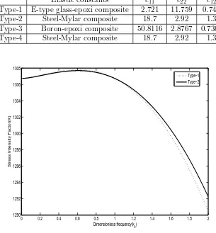
Table 1. Engineering elastic constants

Elastic constants c11 c22 c12

Type-1 E-type glass-epoxi composite 2.721 11.759 0.741 Type-2 Steel-Mylar composite 18.7 2.92 1.3 Type-3 Boron-epoxi composite 50.8116 2.8767 0.7364 Type-4 Steel-Mylar composite 18.7 2.92 1.3

0 0.2 0.4 0.6 0.8 1 1.2 1.4 1.6 1.8 2 1290

1292 1294 1296 1298 1300 1302 1304 1306 1308

Dimensionless frequency(k_s)

Stress Intensity Factor(K)

Type−1 Type−2

0 0.2 0.4 0.6 0.8 1 1.2 1.4 1.6 1.8 2 116

118 120 122 124 126 128 130 132

Dimensionless frequency(k_s)

Stress Intensity Factor(K)

Type−3 Type−4

Fig.3 SIF versus Frequency

From the Fig. 2- Fig. 3, it is clear that the SIF decreases with the increasing value of the frequency for any pair of materials selected. For large value of frequency the SIF diminishes and tends to zero which also can be observed from the expression of the SIF given by the equation (42). The effect of material constants on the SIF is also significant here. It has been observed that the values of the SIF change if the materials are interchanged. That difference depends on the elastic constants of the materials.

0.1 0.2 0.3 0.4 0.5 0.6 0.7 0.8 0.9 1 1.1 0

10 20 30 40 50 60 70 80 90 100

x

Crack Opening Displacement (COD)

k_s=0.72 k

s=0.76

k

s=0.80

k_s=0.68 Type−1

Type−2

Type−3

Type−4

Fig.4 Crack Opening Displacement

increases gradually from zero, attains maximum value and then decreases to zero. It is found that the values of COD increases (Fig. 4) for different types of material constants. In all cases the variation of COD is found to be prominent for different orthotropic materials.

VII. Conclusion

An interfacial crack problem with a Griffith Crack between two dissimilar orthotropic media has been solved and numerical computation has been done with a pair of composite materials. The SIF(K) and COD have been obtained at the tip of the crack at the orthotropic bi-material interface subject to P wave incidence. The singularities and discontinuities associated with the incidence P waves and crack have been predicted in the solution. The graphs of Stress Intensity Factor and Crack Opening Displacement have been plotted to show the effects of various parameters on these quantities. The graph of stress intensity factor against the dimensionless frequency initially increases with increasing value of frequency (ks) and after

attaining maximum value it decreases and finally tending to zero. The COD has been plotted for different value of frequency (ks). The Crack Opening Displacement first increases and

then decreased rapidly with increase in frequencyks and finally tending to 1. From the all

graphs it can be concluded that the values of SIF and COD can be controlled and arrested within a certain range by monitoring applied loads.

Acknowledgement

This research work is financially supported by The University Grant Commission Rajiv Gandhi National Fellowship(UGC RGNF) , New Delhi, India.

References

[1] P. Basak, S. C. Mandal, “P-wave Interaction by an Asymmetric Crack in an Orthotropic Strip”, Int. J. Appl. Comput. Math., vol. 1, pp. 157-170, 2015.

[2] S. Das, B. Patra, L. Debnath, “Diffraction of SH-Waves by a Griffith crack in an infinite Transver-sly Orthotropic Medium”, Appl. Math.Lett., vol. 12, pp. 57-61, 1999.

[3] S. Das, S. Mukhopadhyay, R. Prasad, “Stress intensity factor of an edge crack in bonded or-thotropic materials” Int. J. Fract., vol. 168, no. 1, pp. 117-123, 2011.

[4] J. De, B. Patra, “Edge Crack in Orthotropic Elastic half-plane”, Ind. J. Pure Appl. Math., vol. 20, no. 9, pp. 923-930, 1989.

[5] S. H. Ding, X. Li, “The collinear crack problem for an orthotropic functionally graded coating-substrate structure”,Arch. Appl. Mech., vol. 84, pp. 291-307, 2014.

[6] A. C. Garg, “Stress distribution near periodic cracks at the interface of two bonded dissimilar orthotropic half planes”,Int. J. Eng. Sci., vol. 19, pp. 1101-1114, 1981.

[7] S. Itou, “Diffraction of an antiplane shear wave by two coplanar Griffith cracks in an infinite elastic medium”Int. J. Solids Struct., vol. 16, pp. 1147-1153, 1980.

[8] S. Itou, “Stress Intensity Factors for two parallel interface cracks between a nonhomogenious bonding layerand two dissimilar orthotropic half planes under tension”, Int. J. Fract., vol. 175, pp. 187-192, 2012.

[9] S. Itou, “Dynamic Stress Intensity Factors of Three Collinear Cracks in an Orthotropic Plate Subjected to Time-Harmonic Disturbance”,J. of Mech., vol. 32, no. 5, pp. 491-499, 2016.

[10] D. L. Jain, R. P. Kanwal, “Diffraction of elastic waves by two coplanar Griffith cracks in an infinite elastic medium”, Int. J. Solids Struct., vol. 8, pp. 961-975, 1972.

[12] E. Lira-Vergara, C. Rubio-gonzalez, “Dynamic stress intensity factor of interfacial finite cracks in orthotropic materials”, Int. J. Fract., vol. 135, pp. 285-309, 2005.

[13] E. Lira-Vergara, C. Rubio-gonzalez, “Dynamic stress intensity factor of interfacial finite cracks in orthotropic materials subjected to concentrated loads”, Int. J. Fract., vol. 135, pp. 285-309, 2005.

[14] X. F. Li, “Two perfectly bonded dissimilar orthotropic strips with an interfacial crack normal to the boundaries”, Appl. Math. and Comp., pp. 961-975, 2005.

[15] S. C. Mandal, M. L. Ghosh, “Interaction of elastic waves with a periodic array of coplanar Griffith cracks in an orthotropic medium”, Int. J. Eng. Sci., vol. 32, no. 1, pp. 167-178, 1994.

[16] M. M. Monfared, M. Ayatollahi, “Dynamic stress intensity factors of multiple cracks in an or-thotropic strip with FGM coating”,Eng. Fract. Mech., vol. 109, 45-57, 2013.

[17] S. Mukherjee, S. Das, “Interaction of three interfacial Griffith cracks between bonded dissimilar orthotropic half planes”,Int. J. Solids Struct., vol. 44, pp. 5437-5446, 2007.

[18] M. S. Matbuly, “Analytical solution for an interfacial crack subjected to dynamic anti-plane shear loading”,Acta Mechanics, vol. 163, 77-85, 2006.

[19] P. K. Satapathy, H. Parhi, “Stresses in an orthotropic strip containing a Griffith crack”,Int. J. Eng. Sci., vol. 16, pp. 147-154, 1978.

[20] J. Sarkar, S. C. Mandal,M. L. Ghosh, “Diffraction of elastic waves by three coplaner Griffith cracks in an orthotropic medium”, Int. J. Eng. Sci., vol. 33, no. 2, pp. 163-177, 1995.

[21] S. Sinharoy, “Elastostatic problem of an infinite row of parallel cracks in an orthotropic medium under general loading”,Int. J. Phys. Math. Sci., vol. 3, no. 1, pp. 96-108, 2013.