Solving Transportation Problem by Various
Methods and Their Comaprison
Dr. Shraddha Mishra
Professor and Head
Lakhmi Naraian College of Technology, Indore, RGPV BHOPAL
Abstract: The most important and successful applications in the optimaization refers to transportation problem (tp), that is a special class of the linear programming (lp) in the operation research (or).
Transportation problem is considered a vitally important aspect that has been studied in a wide range of operations including research domains. As such, it has been used in simulation of several real life problems. The main objective of transportation problem solution methods is to minimize the cost or the time of transportation.
An Initial Basic Feasible Solution(IBFS) for the transportation problem can be obtained by using the North-West corner rule, Miinimum Cost Method and Vogel’s Approximation Method. In this paper the best optimality condition has been checked.
Thus, optimizing transportation problem of variables has remarkably been significant to various disciplines.
Key words:
Transportation problem, Linear Programming (LP),
1. Introduction
The first main purpose is solving transportation problem using three methods of transportation model by linear programming (LP).The three methods for solving Transportation problem are:
1. North West Corner Method 2.Minimum Cost Method 3. Vogel’s approximation Method
Trannsportation Model
Transportation model is a special type of networks problems that for shipping a commodity from source (e.g., factories) to destinations (e.g., warehouse). Transportation model deal with get the minimum-cost plan to transport a commodity from a number of sources (m) to number of destination (n).
Let si is the number of supply units required at source i (i=1, 2, 3... m), dj is the number of demand units required at destination j (j=1, 2,3... n) and cij represent the unit transportation cost for transporting the units from sources i to destination j.
Using linear programming method to solve transportation problem, we determine the value of objective function which minimize the cost for transporting and also determine the number of unit can be transported from source i to destination j. If xij is number of units shipped from source i to destination j.
The objective function
minimize Z=
m i
n j
c
1 1
ij xij
Subject to
n
j 1xij = si for i=1,2,...m.
m
i 1xij= dj for j= 1,2,....n.
And xij ≥ 0 for all i to j.
A transportation problem said to be balanced if the supply from all sources equals the total demand in all destinations
m i
s
1
i =
n j
d
1
j
Otherwise it is called unbalanced.
A transportation problem is said to be balanced if the total supply from all sources equals the total demand in all destinations
Otherwise it is called unbalanced. METHODS FOR SOLVING TRANSPORTATION PROBLEM
There are three methods to determine the solution for balanced transportation problem:
1. Northwest Corner method 2. Minimum cost method
3. Vogel’s approximation method
We present the three methods and an illustrative example is solved by these three methods.
1. North- West Corner Method
The method starts at the Northwest-corner cell (route) of the tableau (variable x11)
(i) Allocate as much as possible to the selected cell and adjust the associated a mounts of supply and demand by subtracting the allocated amount. (ii) Cross out the row or Column with zero supply or demand to indicate that no further assignments can be made in that row or column. If both a row and a column net to zero simultaneously, cross out one only and leave a zero supply (demand in the uncrossed-out row (column).
(iii) If exactly one row or column is left uncrossed out,
stop .otherwise, move to the cell to the right if a column has just been crossed out or below if a row has been crossed out .Go to step (i).
2. Minimum-Cost Method
The minimum-cost method finds a better starting solution by concentrating on the cheapest routes. The method starts by assigning as much as possible to the cell with the smallest unit cost .Next, the satisfied row or column is crossed out and the amounts of supply and demand are adjusted accordingly. If both a row and a column are satisfied simultaneously, only one is crossed out, the same as in the northwest –corner method .Next ,look for the uncrossed-out cell with the smallest unit cost and repeat the process until exactly one row or column is left uncrossed out .
3. Vogel’s Approximation Method (VAM) Vogel’s Approximation Method is an improved
version of the minimum-cost method that generally produces better starting solutions.
(i) For each row (column) determine a penalty measure by subtracting the smallest unit cost element in the row (column) from the next smallest unit cost element in the same row (column).
(ii) Identify the row or column with the largest penalty. Break ties arbitrarily. Allocate as much as possible to the variable with the least unit cost in the selected row or column satisfied row or column. If a row and column are satisfied simultaneously, only one of the two is crossed out, and the remaining row (column) is assigned zero supply (demand).
(iii) (a) If exactly one row or column with zero supply or demand remains uncrossed out, stop. (b) If one row (column) with positive supply
(demand) remains uncrossed out, determine the basic variables in the row (column) by the least- cost method .stop.
(c) If all the uncrossed out rows and columns have (remaining) zero supply and demand, determine the zero basic variables by the least-cost method .stop. ).
(d) Otherwise, go to step (i).
ILLUSTRATIVE EXAMPLE
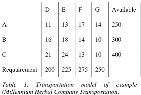
Millennium Herbal Company ships truckloads of grain from three silos to four mills . The supply (in truckloads) and the demand (also in truckloads) together with the unit transportation costs per truckload on the different routes are summarized in the transportation model in table.1.
D E F G Available
A 11 13 17 14 250
B 16 18 14 10 300
C 21 24 13 10 400
Requairement 200 225 275 250
Table 1. Transportation model of example (Millennium Herbal Company Transportation)
The model seeks the minimum-cost shipping schedule between the silos and the mills. This is equivalent to determining the quantity xij shipped from silo i to mill j (i=1, 2, 3; j=1, 2, 3, 4)
1. North West-Corner method
The application of the procedure to the model of the example gives the starting basic solution in table.2. Table 2. The starting solution using Northwest-corner method
Since ai = bj = 950
The Starting basic Solution is given as follows : The first allocation is made in the cell (1,1), the magnitude being x11=min(250,200) = 200. The Second allocation is made in the cell (1,2) and the magnitude of the allocation is given by
Third allocation is made in the cell (2,2) and the magnitude of the allocation is given by
X22 =min(300,225-50) =175
Fourth allocation is made in the cell (2,3) and the magnitude of the allocation is given by
X23 =min(300-175,275) =125.
Fifth allocation is made in the cell (3,3) and the magnitude of the allocation is given by
X33 =min(400,275-125) =150.
Sixth allocation is made in the cell (3,4) and the magnitude of the allocation is given by
X34 =min(400-150,250) =250.
Table 2 T.P. solution using North West corner method
Hence an IBFS to the given TP has been obtained and is displayed in the Table 1.1
The Transportation cost according to the above route is given by
Z=200×11 + 50×13 + 175×18 + 125×14 + 150×13 +2 50×10=12200.
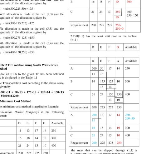
2. Minimum Cost Method
The minimum-cost method is applied to Example (Millennium Herbal Company) in the following manner:
D E F G Available
A 11 13 17 14 250
B 16 18 14 10 300
C 21 24 13 10 400
Requairement 200 225 275 250
1. Cell (3,4) has the least unit cost in the tableau (=10).the most that can be shipped through (3,4) is x12=min (250.,300) =250. which happens to satisfy column 4 simultaneously, we arbitrarily cross out column 4 and adjust in the availability 400-250=50.
D E F G Available
A 11 13 17 14 250
B 16 18 14 10 300
C 21 24 13 250
10
400-250=150
Requairement 200 225 275 250-250=0
2.Cell(1,1) has the least unit cost in the tableau (=11).
D E F G Available
A 200
11
13 17 14 250-200=50
B 16 18 14 10 300
C 21 24 13 10 400
Requairement 200 225 275 250
the most that can be shipped through (1,1) is x11=min (200.,250) =200. which happens to satisfy column 1 simultaneously, we arbitrarily cross out column 1 and adjust the in availablility 250-200=50.
3.Continuing in the same manner ,we successively assign Cell (1,2) has the least unit cost in the tableau (=13).the most that can be shipped through (1,2) is x12=min (225.,50) =50. which happens to satisfy row 1 simultaneously, we arbitrarily cross out row 1 and adjust the in requairement 225-50=175.
D E F G Available
A 200
11 50 13
17 14 250
B 16 175
18 125 14
10 300
C 21 24 150
13 250 10
400
D E F G Available
A 11 50
13
17 14 50-50=0
B 16 18 14 10 300
C 21 24 13 10 400
Requairement 200 225-50=175
275 250
4. Continuing in the same manner ,we successively assign Cell (3,3) has the least unit cost in the tableau (=13).the most that can be shipped through (3,3) is x33=min (275.,400) =275. which happens to satisfy column 3 simultaneously, we arbitrarily cross out column 3 and adjust the in availability 400-275=125.
D E F G Available
A 11 13 17 14 50
B 16 18 14 10 50
C 21 24 150
13
10
150-150=0
Requairement 200 175 275-150=125
250
5.Continuing in the same manner ,we successively assign Cell (2,2) has the least unit cost in the tableau (=18).the most that can be shipped through (2,2) is x22=min (50.,175) =50. which happens to satisfy row 2 simultaneously, we arbitrarily cross out row 2 and adjust the in requairement 175-50=125..
D E F G Available
A 11 13 17 14 50
B 16 175
18
14 10 300-175=125
C 21 24 13 10 125
Requairement 200 175-50=125
275 250
6.. Continuing in the same manner ,we successively assign Cell (3,2) has the least unit cost in the tableau (=24).the most that can be shipped through (3,2) is x32=min (125.,125) =125. which happens to satisfy row 3 simultaneously, we arbitrarily cross out row 3
D E F G Available
A 11 13 17 14 50
B 16 175
18
14 10 175
C 21 24 13 10 125
Requaireme nt
200
175-175=0
275 250
The final T.P. rout
D E F G Available
A 200
11
50
13
17 14 250
B 16 175
18
125
14
10 300
C 21 24 150
13
250
10
400
Requaireme nt
200 225 275 250
The Transportation cost according to the above route is given by
Z=200×11 + 50×13 +175×18 + 125×14 + 150×13 +250×10 =12200.
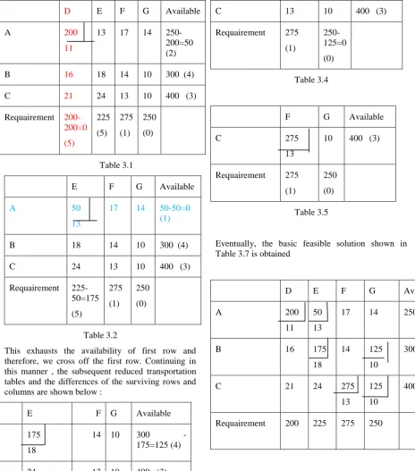
3. Vogel’s Approximation Method (VAM)
D E F G Available
A 200
11
13 17 14 250- 200=50 (2)
B 16 18 14 10 300 (4)
C 21 24 13 10 400 (3)
Requairement 200-200=0
(5)
225 (5)
275 (1)
250 (0)
Table 3.1
E F G Available
A 50
13
17 14 50-50=0 (1)
B 18 14 10 300 (4)
C 24 13 10 400 (3)
Requairement 225-50=175 (5)
275 (1)
250 (0)
Table 3.2
This exhausts the availability of first row and therefore, we cross off the first row. Continuing in this manner , the subsequent reduced transportation tables and the differences of the surviving rows and columns are shown below :
E F G Available
B 175
18
14 10 300
-175=125 (4)
C 24 13 10 400 (3)
Requairement 175-175=0(6)
275 (1)
250 (0)
Table 3.3
F G Available
B 14 125 125-125=0
(4)
C 13 10 400 (3)
Requairement 275 (1)
250-125=0 (0)
Table 3.4
F G Available
C 275
13
10 400 (3)
Requairement 275 (1)
250 (0)
Table 3.5
Eventually, the basic feasible solution shown in Table 3.7 is obtained
D E F G Available
A 200
11 50 13
17 14 250
B 16 175
18
14 125 10
300
C 21 24 275
13
125 10
400
Requairement 200 225 275 250
The transportation cost according to this route is given by
Z=200×11 + 50×13 + 175×18 + 125×10 + 275×13 +12 5×10=12075.
VAM produces a better starting Solution. This cost is less than northwest-corner method COMPARISON BETWEEN THE THREE METHODS
corner method is quick solution because computations take short time but yields a bad solution because it is very far from optimal solution. Vogel's approximation method and Minimum-cost method is used to obtain the shortest road. Advantage of Vogel’s approximation method and Minimum-cost method yields the best starting basic solution because gives initial solution very near to optimal solution but the solution of Vogel’s approximation methods is slow because computations take long time. The cost of transportation with Vogel's approximation method and Minimum-cost method is less than North-West corner method.
The cost of transportation is less than North-west corner method.
CONCLUSION
The result in three methods are defferent. The decision maker may choose the optimal result of the running of the three program (minimum) and determined the number of units transported from source i to destination j.
REFERENCES
[1] Kanti Swarup ,P. K. Gupta ,Man Mohan . “Operation Research”, Sultan Chand & Sons, New Delhi,2005. [2] Hamdy A.Taha.” Operations Research: An Introduction
“,Prentice Hall, 7 editions 5 ,USA,2006.