The Thirty-Third AAAI Conference on Artificial Intelligence (AAAI-19)
Joint Semi-Supervised Feature Selection
and Classification through Bayesian Approach
Bingbing Jiang,
1Xingyu Wu,
1Kui Yu,
2Huanhuan Chen
1∗1School of Computer Science and Technology, University of Science and Technology of China, Hefei, China.
2School of Computer and Information, Hefei University of Technology, Hefei, China.
{jiangbb, xingyuwu}@mail.ustc.edu.cn, [email protected], [email protected].
Abstract
With the increasing data dimensionality, feature selection has become a fundamental task to deal with high-dimensional data. Semi-supervised feature selection focuses on the prob-lem of how to learn a relevant feature subset in the case of abundant unlabeled data with few labeled data. In re-cent years, many semi-supervised feature selection algo-rithms have been proposed. However, these algoalgo-rithms are implemented by separating the processes of feature selection and classifier training, such that they cannot simultaneously select features and learn a classifier with the selected fea-tures. Moreover, they ignore the difference of reliability in-side unlabeled samples and directly use them in the train-ing stage, which might cause performance degradation. In this paper, we propose a joint semi-supervised feature se-lection and classification algorithm (JSFS) which adopts a Bayesian approach to automatically select the relevant fea-tures and simultaneously learn a classifier. Instead of using all unlabeled samples indiscriminately, JSFS associates each un-labeled sample with a self-adjusting weight to distinguish the difference between them, which can effectively eliminate the irrelevant unlabeled samples via introducing a left-truncated Gaussian prior. Experiments on various datasets demonstrate the effectiveness and superiority of JSFS.
Introduction
In many real-world applications, such as scene classifica-tion, text categorizaclassifica-tion, gene expression data analysis, the data dimensionality becomes larger and larger. Directly us-ing these high-dimensional data might lead to lower time ef-ficiency and performance deterioration due to the existence of noisy or irrelevant features. As a dimensionality reduction technique, feature selection tries to find a lower-dimensional representation of data via removing irrelevant features with-out altering the original feature space (Chandrashekar and Sahin 2014). Due to its effective representation and bet-ter inbet-terpretability for data, various feature selection al-gorithms have been proposed (He, Cai, and Niyogi 2006; Zhao and Liu 2007; Nie et al. 2010; Jiang et al. 2016).
According to the availability of class label, the existing feature selection algorithms can be divided into three differ-ent groups: unsupervised, supervised and semi-supervised
∗
Corresponding author: Huanhuan Chen.
Copyright c2019, Association for the Advancement of Artificial Intelligence (www.aaai.org). All rights reserved.
(Sheikhpour et al. 2017). Without the guidance of class la-bel information, unsupervised algorithms cannot select the features that effectively distinguish different classes. On the other hand, supervised algorithms can select discrimina-tive features with sufficient labeled data. However, the la-beled data is usually scarce since it is expensive and time-consuming to collect them. Therefore, it is of great prac-tical significance to design the feature selection algorithm that can exploit both labeled and unlabeled data simultane-ously. Inspired by the semi-supervised learning (Chapelle, Sch¨olkopf, and Zien 2006; Sakai et al. 2017; Chen, Jiang, and Yao 2018), semi-supervised feature selection has been proposed, which can select features with the help of the la-bel information of lala-beled data and the structure information of unlabeled data.
To learn the relevant features in the case of abundant unla-beled data with few launla-beled data, many state-of-the-art semi-supervised feature selection algorithms have been proposed. Most semi-supervised feature selection algorithms are filter-based, which are implemented by ranking the features based on their capability of maintaining the specific data struc-ture or some information criterion. For example, Zhaoet al
proposed a locality sensitive discriminant algorithm (Zhao, Lu, and He 2008), which selects the features that can max-imize the margin between different classes and simultane-ously preserve the similarity between data. Based on the trace ratio criterion in supervised learning (Nie et al. 2008), Liuet aldesigned a semi-supervised feature selection algo-rithm that can avoid selecting the features with very small variance (Liu et al. 2013). However, the filter-based semi-supervised feature selection algorithms ignore the interac-tion between the selecinterac-tion of feature and the learning tasks. Therefore, it is difficult for them to select the features that are particularly effective for a given learning algorithm (Xu et al. 2010).
selec-tion algorithm. Luoet al.usedl2q-norm (0 < q ≤1) con-straint to replace thel21-norm and designed an insensitive sparse regression algorithm (Luo et al. 2018). Unfortunately, this algorithm has at least four free parameters that need to be tuned, which makes it difficult to be practical. Generally, although the embedded algorithms integrate the feature se-lection process to the training, they are not able to adaptively select features and simultaneously learn a classifier with the selected features. Concretely, they need to predetermine the number of selected features and then select features accord-ing to the feature projection matrix. To validate the effec-tiveness of selected features, an additional classifier (usu-ally SVM or KNN) is required to train a classifier by using the selected features. Sometimes, they could still perform well by using a classifier with tuned parameters even though including some irreverent features. Therefore, it is hard to judge whether their promising performance is attributed to the robust classifier or the selected features.
Moreover, the filter-based or embedded semi-supervised feature selection algorithms mentioned above indiscrimi-nately and directly use the labeled and unlabeled samples to design the evaluation criterion or objective functions for selecting features. In fact, the labeled samples are usually more reliable while there might inevitably exist noisy unla-beled samples since abundant unlaunla-beled samples could be collected from different resources. Therefore, using all un-labeled samples indiscriminately could have an adverse im-pact on the feature selection and even lead to performance degradation. Although the semi-supervised feature selection has been used to some applications, it fails to take the ro-bustness to the noisy unlabeled samples into consideration.
To alleviate this issue, Changet al. proposed a convex semi-supervised feature selection algorithm (Chang et al. 2014), which preassigns different scores for labeled and un-labeled samples. However, this algorithm lacks the ability to capture the local geometric structure of unlabeled data. In fact, the local geometric structure refers to the local neigh-borhood relationship, which is very effective for feature se-lection especially when very few labeled samples with the high-dimension feature are provided (Liu et al. 2014). More-over, it determines the scores of labeled and unlabeled sam-ples empirically, making it hard to be useful. Thus, it is of vi-tal importance for semi-supervised feature selection to make full use of unlabeled samples and simultaneously take an ef-fective strategy to distinguish their difference of reliability.
Motivated by the aforementioned issues, we propose a novel semi-supervised feature selection algorithm, called joint semi-supervised feature selection and classification through Bayesian approach (JSFS). The main contributions of this paper are summarized as follows:
• Combining with a Bayesian approach, JSFS is able to adaptively identify the relevant features and simultane-ously learn a classifier with the selected features. Thus, JSFS does not require the number of selected features to be predetermined, nor an additional classifier to be adopted for training, which are two main limitations of the existing semi-supervised feature selection algorithms.
• To make better use of prior knowledge from labeled and
unlabeled samples, we define a prior on feature weight to generate adaptive sparsity in the feature space and then propose an alternative way to optimize the feature weight.
• Instead of using all unlabeled samples indiscriminately and directly, we associate each unlabeled sample with a self-adjusting weight first and then introduce a left-truncated Gaussian prior on it. By this prior, JSFS can eliminate the irrelevant unlabeled samples, improving the robustness against noise.
• JSFS is compared with the state-of-the-art algorithms. The experimental results on different real-world datasets validate the effectiveness and superiority of JSFS.
The proposed algorithm
In this section, we will propose the joint semi-supervised feature selection and classification algorithm in detail.
Notation and Model Specification
In semi-supervised learning, training dataX consists of a labeled dataset with l samples, Xl = {xi}li=1 associated with class labelsy= [y1, . . . , yl]T, and an unlabeled dataset with usamples, Xu = {xi}in=l+1, where xi ∈ Rd and
n = l +uis the total number of training samples. This paper studies the binary semi-supervised feature selection problem, in which the class label yi ∈ {0,1}. Given the training data, the main aim is to learn a prediction model based on the selected features, which can make an accurate prediction for out-of-sample data.
The prediction model adopted by previous feature selec-tion algorithms is a linear combinaselec-tion of all features, treat-ing the labeled and unlabeled samples equally in the traintreat-ing stage. This model is improper due to ignoring the quality difference between labeled and unlabeled samples and the difference between unlabeled samples themselves. To over-come this limitation, we propose a separable linear model from training data as:
f(X,w,Λ) =ΛXw, (1)
whereX = [x1,· · ·,xn]T ∈ Rn×d denotes training sam-ples,w = [w1,· · ·, wd]T is thed-dimensional weight vec-tor for the feature, and Λ = diag(λ1, . . . , λn)denotes an
Priors over Weights of Features and Samples
In semi-supervised classification, the discriminant informa-tion included in labeled samples is very limited. To exploit abundant unlabeled samples, previous semi-supervised al-gorithms define an additional regularizer to capture the local geometric structure underlying the unlabeled samples. From a Bayesian perspective, the regularizer is corresponding to the prior knowledge (Bishop 2006; Jiang et al. 2017). To make better use of few labeled and abundant unlabeled sam-ples, a sparseness-promoting prior over above feature weight vectorwis designed as:
p(w|α) = (2π)−d2|A+B| 1
2exp−1 2w
T(A+B)w , (2)
whereα= [α1, . . . , αd]is ad-dimensional hyper-parameter vector, andB =γXTLX, in whichγ(γ≥0)is a prede-termined parameter that controls the use of local geometric structure of training samples, andLis the graph Laplacian that characterizes the intrinsic local structure. By combin-ing matrix B with feature weight vector w, we can inte-grate the local geometric structure into the prior and conduct semi-supervised feature selection within a Bayesian frame-work. Note that when the local structure is not obvious, the
γ will have a very small value, making matrix B possi-bly singular. At this point, the prior in Eq. (2) is close to a zero-mean Gaussian prior with the inverse covariance ma-trixA = diag(α1, . . . , αd). Therefore, introducing a non-negative diagonal matrixAthat acts as a sparse regularizer, could stabilize the prior especially whenBmay be singular. To capture the local neighborhood relationship of training samples, the graph Laplacian matrixL=D−Sis built.S
is an affinity matrix whose elementSijreflects the similarity between samplesxiandxj, andDdenotes a diagonal ma-trix with the diagonal elementDii =PjSij. To efficiently compute the graph Laplacian, we use ak-nearest neighbor graph to construct the affinity matrixSas follows:
Sij=
η ifxiandxjhave the same label, 1 ifxiorxjis unlabeled
butxi∈kN N(xj) orxj ∈kN N(xi), 0 otherwise
(3)
wherekN N(xj)denotes theknearest neighbors set of sam-plexj, andη is a constant which is set as 10 in this paper. The affinity matrixS measures the neighborhood relation-ship of training data while considering the difference be-tween the samples with the same label and the unlabeled samples that are sufficiently close to each other.
Sample weights reflect the importance of unlabeled sam-ples. For important unlabeled samples, the corresponding weights should have relatively large values and vice versa. To avoid the indiscriminative use of unlabeled samples and simultaneously ensure λj ≥ 0, a left truncated Gaussian prior is introduced over unlabeled sample weights
p(λ|c) = n
Y
j=l+1
p(λj|cj) = n
Y
j=l+1
Nt(λj|0, c−j1), (4)
where λ = [λl+1, . . . , λn]T is the weight vector of un-labeled samples, cj is the inverse of variance which is
also referred as a hyper-parameter, cis the corresponding hyper-parameter vector andNt(λj|0, c−j1) denotes the left truncated Gaussian distribution. For each unlabeled sample weightλj(j =l+ 1, . . . , n), its prior is formalized as fol-lows
p(λj |cj) =
2N(λj |0, c−j1) ifλj≥0
0 otherwise
= 2N(λj |0, cj−1)·δ(λj), (5)
whereδ(λj)is an indicator function that returns1for each
λj ≥ 0 and 0 otherwise. According to (Chen, Tiˇno, and Yao 2009; 2014), this truncated Gaussian prior can gener-ate adaptive sparseness in the estimation ofλ.
In Bayesian research (Tipping 2001; Li and de Rijke 2018), the non-informative Gamma distribution is often in-troduced as hyperpriors for hyper-parameters αi and cj, which can promote the sparsity of feature and unlabeled sample space. Specifically, the posterior estimate of the pa-rameter (wiorλj) will be very close to zero for a large value of hyper-parameter, thus the corresponding feature or unla-beled sample will be removed from the current model due to less contribution.
Optimization
Based on the prediction model in Eq. (1), the posterior prob-ability for samplexibelonging to positive class can be cal-culated by applying a logistic sigmoid function σ(x) = 1/(1 +e−x) to its prediction, i.e.,p(y
i = 1|xi,w, λ) =
σ(λiwTxi). Also, the posterior probability for negative class,p(yi = 0|xi,w, λ) = 1−σ(λiwTxi). By providing pseudo labels for unlabeled samples, the likelihood function
p(y|X,w,λ)can be decomposed as:
p(y|X,w,λ) =p(yl|X,w,λ)·r p(yeu|X,w,λ), (6)
wherep(yl|X,w,λ)denotes the likelihood function on la-beled samples with true label vector yl = [y1, . . . , yl]T,
p(yeu|X,w,λ)denotes the likelihood function on unlabeled samples with pseudo label vector yeu = [yel+1, . . . ,yen]T, andy= [yl,yeu]
T. To enlarge the label information, we
in-troduce pseudo labelsyej for unlabeled samples, which can be obtained by the label propagation algorithm (Zhou et al. 2004). The pseudo labels extend the definition of likelihood, but also contain some false labels for unlabeled samples, which affects the reliability of likelihood. Therefore, a trade-off parameterris introduced to balancep(yl|X,w,λ)and
p(yeu|X,w,λ).
The MAP Estimates of Parameters w andλ: Having the priors and likelihood, the posterior distribution overw
andλcan be computed by using the Bayesian rule:
p(w,λ|y,α,c) = p(w|α)p(λ|c)p(y|X,w,λ)
p(y|X,α,c) . (7)
Due to the non-Gaussian distribution of the likelihood,
p(y|X,α,c) = R R
p(w|α)p(λ|c)p(y|X,w,λ)dwdλ
distribution for likelihood and putting the priors in Eqs. (2) and (4) into the log of posteriorp(w,λ|y,α,c), we have
Q(w,λ) = logp(w|α) + logp(λ|c) + logp(y|X,w,λ)
= l X
i=1
[yilogσi+ (1−yi) log(1−σi)]
+µ
n X
j=l+1
[yje logσj+ (1−eyj) log(1−σj)]
−1
2w
T(A+B)w−1
2λ
TCλ+
n X
j=l+1
logδ(λj),
(8)
whereσi =σ(λiwTxi),µ= lnr(0≤µ≤1)is a param-eter that controls the importance of the likelihood function defined on unlabeled samples, and C=diag(cl+1, . . . , cn). As the indicator functionδ(λj)is not differentiable, we can approximate it by a sigmoid functionσ(βλj)withβ = 5. The maximum a posterior (MAP) estimates ofwandλcan be boiled down to how to maximizeQ(w,λ). Due to the non-convexity of the likelihood, it is difficult to maximize
Q(w,λ)with respect to parameterswandλdirectly and si-multaneously. To solve this maximization problem, we pro-pose an alternative way to optimizeQ(w,λ)with respect to one parameter assuming the other to be fixed.
To find the MAP estimatewb, we first optimizeQ(w,λ) with respect towwhenλis fixed. We adopt the iteratively re-weighted least squares method to updatewas follows:
b
wnew =wb−Hw−1gw, (9)
wheregwdenotes the gradient vector of Q(w,λ)with re-spect tow, andHwis the Hessian matrix. Whenλis fixed,
Q(w,λ)can be written asQ(w|λ). Therefore, the gradient
gwis given by:
gw=
∂Q(w|λ)
∂w =X
T
e
Λ(y−σ)−(A+B)w, (10)
whereΛe is a diagonal matrix withΛeii = 1ifxiis labeled andΛeii=µλiotherwise, andσ= [σ1, . . . , σn]T. The Hes-sian matrix ofwis given by:
Hw=
∂2Q(w|λ)
∂w2 =−(X
TEX+A+B), (11)
whereEis ad×ddiagonal matrix withEii =σi(1−σi) ifxiis labeled andEii =µλi2σi(1−σi)otherwise.
Likewise, we updateλwith fixedwas follows:
b
λnew =λb−Hλ−1gλ, (12)
wheregλ denotes the gradient vector ofλ, and Hλ is the corresponding Hessian matrix. The gradientgλis given by:
gλ=
∂Q(λ|w)
∂λ =µP(yeu−σu)−Cλ+kλ, (13)
wherekλ = [β(1−σ(βλl+1)), . . . , β(1−σ(βλn))]T and
σu = [σl+1, . . . , σn]T areu-dimensional vectors,P is an
u×udiagonal matrix with thei-th diagonal elementsPii=
wTx
l+i. Then, the Hessian matrix ofλis given by:
Hλ=
∂2Q(λ|w)
∂λ2 =−(µP
TE
uP+C+O), (14)
whereEu andOareu×udiagonal matrices with theiri -th diagonal elements Eu,ii = σl+i(1−σl+i), and Oii =
β2σ(βλ
l+i)(1−σ(βλl+i)).
Based on the above alternative update rules, the MAP es-timates of feature weightswand unlabeled sample weights
λcan be obtained. Provided with the MAP estimates of pa-rameters, we can update hyper-parametersαandc.
Algorithm 1The proposed JSFS algorithm
1: Input:Training dataX ∈Rn×d, parametersγandµ.
2: Output: The selected feature indexes and their corre-sponding weight vectorwfor the linear classifier.
3: Initializewi,λj,αi, andcj for i = 1, . . . , dandj =
l+ 1, . . . , n.
4: Construct the affinity matrixSand graph LaplacianL.
5: Obtain the pseudo label vectoryeuvia label propagation.
6: Whilemaxi|wnewi −wiold|>10−3 do
7: Ifkgwk/d <10−3then
8: Fixλ, computegwandHwby Eqs . (10) and (11), and updatew←w−Hw−1gw;
9: end if
10: Remove thei-th feature if|wi|<10−3;
11: Ifkgλk/u <10−3then
12: Fixw, computegλandHλby Eqs . (13) and (14), and updateλ←λ−Hλ−1gλ;
13: end if
14: Remove thej-th unlabeled sample if|λj|<10−3;
15: Updateαandcusing Eqs. (18) and (20);
16: end while
Optimizing the Hyper-parameters αandc: Given the MAP estimate of parametersw andλ, the learning objec-tive becomes the optimization of hyper-parameters α and
c, which boils down to maximize the hyper-parameter pos-terior, i.e.,p(α,c|X,y)∝ p(y|X,α,c)p(α)p(c). Due to the noninformative hyperpriors overαandc, we need only maximize p(y|X,α,c), which is known as the marginal likelihood. Therefore, we can update hyper-parameters by
(αb,cb) = arg max
(α,c)p(y|X,α,c)
= arg max (α,c)
Z Z
p(y|X,w,λ)p(w|α)p(λ|c)dwdλ.
(15)
Since the integral in Eq. (15) is intractable, the maximiza-tion with respect toαandccannot be simultaneously de-rived. To update the hyper-parameters, we use an iterative re-estimation method to alternately optimize the marginal likelihood betweenαandc. First, we attempt to maximize the marginal likelihood with respect toαassumingcto be fixed. Then we haveαb = arg maxαL(α), where
L(α) = Z
p(y|X,w,λ)p(w|α)dw
≈p(y|X,wb,λ)p(wb|α)(2π)d2| −H b
w|−
1 2 ,
(16)
wherewb is the MAP estimate ofw, and H b
likelihood withwb, we have the log marginal likelihood
logL(α)≈logp(y|X,wb,λ)−1 2wb
TA
b w
+1
2log|A+B| − 1
2log| −Hwb|.
(17)
To find the α that can maximize this approximation of log marginal likelihood, we set the first order derivative of logL(α)to zero, and get the update rule
αnewi = 1
b w2
i +Gii+ Σw,ii
, (18)
wherewbi is thei-th element ofwb,Gii is thei-th diagonal element of the matrixG=A−1B(I+A−1B)−1A−1, and Σw,iidenotes thei-th diagonal element of−H−1
b
w .
Likewise, we maximize the marginal likelihood with re-spect tocwhenαis fixed, i.e.,cb= arg maxcL(c), where
L(c)≈p(y|X,w,λb)p(λb|c)(2π)
u
2| −H
b
λ|
−1
2, (19)
whereλb is the MAP estimate ofλ, andH b
λis the Hessian matrix computed atλb. Setting the first order derivative of logL(c)to zero, we have
cnewj = 1
b λ2
j+ Σλ,jj
, (20)
wherebλjis thej-th element ofbλ, andΣλ,jjdenotes thej-th diagonal element of−H−1
b
λ .
With the above update formulas, the pseudo code of the proposed JSFS algorithm is provided as Algorithm 1. Specifically, JCFS first finds the MAP estimatorwb andλb
given the hyper-parametersαi andcj by iteratively using Eqs. (9) and (12), and then updates the hyper-parameters by Eqs. (18) and (20). During updating, we generally find that most ofwiandλjtend to zero, thus the corresponding irrel-evant feature and unlabeled sample will be automatically re-moved from the current model through Bayesian automatic relevance determination (Bishop 2006), which avoids pre-determining the number of selected features and simultane-ously accelerates the training speed. Except for measuring the importance of features, the feature weights w can be used to learn a direct classifier for the samples represented by the selected features. For any unseen samplexˆ, its label ˆ
y = 1wheneverf( ˆx,w) = wTxˆ ≥ 0, andyˆ = 0 when-everf( ˆx,w) = wTxˆ <0. Thus, JSFS does not require an additional classifier to be adopted for training as well.
Experiments
In this section, we conduct a series of experiments to eval-uate the effectiveness of JSFS. The first experiment aims to validate the robustness of JSFS against noisy features and unlabeled samples. Then, eight high-dimensional datasets from various domains are used to verify the performance of classification and feature selection of JSFS.
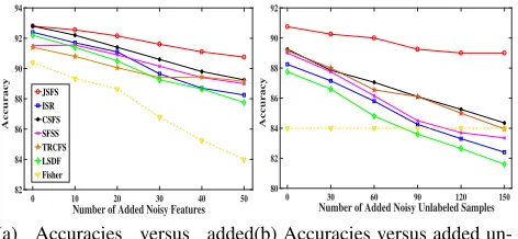
0 10 20 30 40 50
Number of Added Noisy Features
82 84 86 88 90 92 94
Accuracy
JSFS ISR CSFS SFSS TRCFS LSDF Fisher
(a) Accuracies versus added noisy features
0 30 60 90 120 150
Number of Added Noisy Unlabeled Samples
80 82 84 86 88 90 92
Accuracy
(b) Accuracies versus added un-labeled noise samples
Figure 1: Accuracies (in %) of different algorithms with the increase of noisy features and unlabeled samples in data.
Experimental Setup
To illustrate the effectiveness and superiority of JSFS, it is compared with some state-of-the-art feature selection al-gorithms, including three embedded semi-supervised fea-ture selection algorithms: semi-supervised feafea-ture selection via insensitive sparse regression (ISR) (Luo et al. 2018), structural feature selection with sparsity (SFSS) (Ma et al. 2012) and convex semi-supervised feature selection (CSFS) (Chang et al. 2014), two filter-based semi-supervised feature selection algorithm: locality sensitive discriminant feature (LSDF) (Zhao, Lu, and He 2008) and semi-supervised fea-ture selection with trace ratio criterion (TRCFS) (Liu et al. 2013), and one supervised feature selection algorithm: fisher score (Fisher) (Bishop and others 1995).
For a fair comparison, the regularization or trade-off parameters of all comparing algorithms are tuned from {10−2,10−1,· · ·,102}by grid search, the number of near-est neighborkis set as five for all algorithms, and parameters
µandγ ∈ [0,1]for JSFS. Since the comparing algorithms are not able to select features and simultaneously learn a classifier with the selected features. To evaluate the qual-ity of selected features, the linear Support Vector Machine (SVM) (Chang and Lin 2011) is adopted to compute their classification accuracies. Specifically, we first apply these feature selection algorithms to select features and then use SVM to train a classifier with the selected features. For each comparing algorithm, we report their best classification ac-curacies on the test samples represented by the selected fea-tures, employing the trained classifier.
Robustness Against Noisy Features and Samples
The first experiment is to verify the robustness of JSFS against the increasing scales of noisy features and unlabeled samples. We use G50C dataset (Chapelle and Zien 2005), containing 550 samples with two classes, in which each sample has 50 features generated by a 50-dimensional multi-variate Gaussian distribution. G50C is randomly partitioned by 350 samples for training and 200 for testing, in which the training set includes20labeled samples for each class.
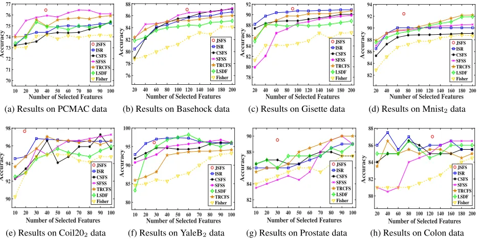
dis-10 20 30 40 50 60 70 80 90 100 Number of Selected Features 70 71 72 73 74 75 76 77 Accuracy JSFS ISR CSFS SFSS TRCFS LSDF Fisher
(a) Results on PCMAC data
20 40 60 80 100 120 140 160 180 200
Number of Selected Features 76 78 80 82 84 86 88 Accuracy JSFS ISR CSFS SFSS TRCFS LSDF Fisher
(b) Results on Basehock data
20 40 60 80 100 120 140 160 180 200
Number of Selected Features
78 80 82 84 86 88 90 92 Accuracy JSFS ISR CSFS SFSS TRCFS LSDF Fisher
(c) Results on Gisette data
20 40 60 80 100 120 140 160 180 200
Number of Selected Features
82 84 86 88 90 92 94 Accuracy JSFS ISR CSFS SFSS TRCFS LSDF Fisher
(d) Results on Mnist2data
10 20 30 40 50 60 70 80 90 100 Number of Selected Features 90 92 94 96 98 Accuracy JSFS ISR CSFS SFSS TRCFS LSDF Fisher
(e) Results on Coil202data
10 20 30 40 50 60 70 80 90 100 Number of Selected Features 80 85 90 95 100 Accuracy JSFS ISR CSFS SFSS LSDF TRCFS Fisher
(f) Results on YaleB2data
10 20 30 40 50 60 70 80 90 100 Number of Selected Features 82 84 86 88 90 Accuracy JSFS ISR CSFS SFSS TRCFS LSDF Fisher
(g) Results on Prostate data
20 40 60 80 100 120 140 160 180 200
Number of Selected Features 80 82 84 86 88 Accuracy JSFS ISR CSFS SFSS TRCFS LSDF Fisher
(h) Results on Colon data
Figure 2: Illustration of the accuracy of JSFS and other feature selection algorithms with different scales of selected features.
tributedN(0,1). Each algorithm in independently run on 20 disparate data partitions, and the average classification racy on the test samples is used to evaluate them. The accu-racy variation curves are illustrated in Figure 1, in which Figure 1(a) demonstrates the accuracies of seven feature se-lection algorithms against gradually increasing noisy fea-tures, and Figure 1(b) shows accuracies versus the increas-ing number of noisy unlabeled samples with 50 noisy fea-tures. As shown in Figure 1, all algorithms trend to achieve reduced accuracy with the increase of the noise in data, and JSFS can consistently outperform the state-of-the-art.
Furthermore, from Figures 1(a) and 1(b) we note that the variation trend of accuracy with added noisy features or un-labeled samples is obviously different. Specifically, the ac-curacies of comparing algorithms are slightly reduced with increasing noisy features in Figures 1(a). This result is rea-sonable because they are feature selection algorithms and largely immune to the noisy features. However, their accu-racies as depicted in Figure 1(b) are rapidly deteriorated with the increase of unlabeled samples. The main reason is that they directly use all available unlabeled samples and fail to take the reliability of them into full consideration. Fortu-nately, except for selecting relevant features for classifica-tion, our algorithm provides a selective mode to effectively exploit unlabeled samples via the adopted prior in unlabeled sample space, which can automatically eliminate the noisy unlabeled samples. The results in Figure 1 demonstrate the significant superiority of JSFS in terms of robustness against the added noise in data, especially when there exist noisy un-labeled samples.
Performance on High-dimensional Datasets
To evaluate the effectiveness of our proposed joint semi-supervised feature selection and classification learning
algo-rithm, 8 high-dimensional datasets that are collected from different fields are used, including two text datasets: PA-MAC and Basehock; four image datasets: Gisette, Mnist2, Coil202 and YaleB2; and two biological datasets: Prostate and Colon. Mnist2 is the most challenging binary version of the MNIST dataset, which aims to separate digit 4 from digit 9. Coil202and YaleB2denote the binary version of the Coil20 and extended YaleB datasets, respectively. The goal is to discriminate object 1 from object 2. The detailed char-acteristics of the datasets are summarized in Table 1. Due to different numbers of samples in training set, we randomly sample 5, 5, 5, 5, 10, 20, 20, and 20 labeled samples each class for Coil202, YaleB2, Colon, Prostate, Mnist2, Gisette, Basehock and PCMAC, and the rest of samples in training set are unlabeled. For these comparing feature selection
al-Table 1: Characteristics of 8 experimental data sets.
Data # features # training # test
PCMAC 3,289 1,000 943
Basehock 4,862 1,000 993
Gisette 5,000 3,500 3,500
Mnist2 784 3,782 1,0000
Coil202 1,024 100 144
YaleB2 1,024 100 28
Prostate 5,966 82 20
Colon 2,000 42 20
0 20 40 60 80 100 120 140 160 180 200 Number of Iterations 0
500 1000 1500 2000 2500 3000
# Number of Features
(a)
0 20 40 60 80 100 120 140 160 180 200 Number of Iterations -200
-150 -100 -50 0
Marginal Likelihood of
(b)
0 20 40 60 80 100 120 140 160 180 200 Number of Iterations 0
200 400 600 800
# Number of Unlabeled Samples
(c)
0 20 40 60 80 100 120 140 160 180 200 Number of Iterations -500
-400 -300 -200 -100 0
Marginal Likelihood of c
(d)
Figure 3: Variation curves of the number of features and unlabeled samples selected by our algorithm and the marginal likeli-hood functions in Eqs. (17) and (19) on PCMAC dataset.
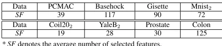
are shown in Figure 2. Different from other feature selec-tion algorithms that require to predetermine the number of selected features, our algorithm can adaptively select rel-evant features and simultaneously remove out the features with less contribution, automatically determining number of selected features. Therefore, the accuracy of JSFS does not vary with increasing number of selected features in Figure 2. Table 2 presents the average number of features selected by JSFS, which demonstrates the sparsity of JSFS.
Table 2: The average number of features selected by JSFS.
Data PCMAC Basehock Gisette Mnist2
SF 39 117 90 72
Data Coil202 YaleB2 Prostate Colon
SF 19 28 30 125
* SFdenotes the average number of selected features.
As shown in Figure 2, the semi-supervised feature selec-tion algorithms achieve higher accuracies than the super-vised algorithm (i.e., Fisher) in most of cases, which vali-dates the usefulness of unlabeled samples for performance improvement. Since our algorithm can perform feature se-lection and simultaneously learn an optimal classifier with the selected features, together with taking the difference of importance between unlabeled samples into consideration. From Figure 2, we observe that our algorithm outperforms other algorithms on 4 out of 8 datasets and also achieves very competitive accuracies on the remaining datasets in compar-ison with the state-of-the-art algorithms.
Complexity and Convergence Analysis
In the initial training stage, our algorithm contains labeled and all available unlabeled samples. The main computa-tional cost of our algorithm is to update the weights of fea-ture and unlabeled samples in Eqs. (9) and (12), which re-quires to use the Cholesky decomposition to compute the inverse of their corresponding Hessian matrices in Eqs. (11) and (14). Therefore, the computational complexity of JSFS isO(d3+u3), in whichdandudenote the number of fea-tures and unlabeled samples, respectively.
Due to the adaptive sparsity in feature and unlabeled sam-ple space, most ofwi andλj will be restricted to a small
neighborhood around 0 and then we remove their corre-sponding features and unlabeled samples in future itera-tions. As iteration goes on,dandurapidly decrease to rel-atively small values in the first few iterations, resulting in
O(¯u3 + ¯d3)computational complexity, where d¯ dand ¯
uu. In fact, our proposed algorithm is efficient with fast convergence. To illustrate the speed of convergence, Figure 3 provides the variation curves of the number of features and unlabeled samples selected by JSFS and their correspond-ing marginal likelihoods on PCMAC dataset. From this fig-ure, we can observe that our proposed algorithm can con-verge stably in the first40iterations, which can accelerate the training speed and guarantee the efficiency for practical applications.
Conclusion
Acknowledgments
This work was supported in part by the National Key Re-search and Development Program of China under Grant 2016YFB1000905, and in part by the National Natural Sci-ence Foundation of China under Grant 91546116, Grant 91846111, Grant 61876206, and Grant 91746209.
References
Belkin, M.; Niyogi, P.; and Sindhwani, V. 2006. Manifold regularization: A geometric framework for learning from la-beled and unlala-beled examples.Journal of Machine Learning Research7:2399–2434.
Bishop, C., et al. 1995. Neural networks for pattern recog-nition. Oxford university press.
Bishop, C. M. 2006. Pattern Recognition and Machine Learning. Springer.
Chandrashekar, G., and Sahin, F. 2014. A survey on fea-ture selection methods. Computers & Electrical Engineer-ing40(1):16–28.
Chang, C.-C., and Lin, C.-J. 2011. LIBSVM: a library for support vector machines. ACM Transactions on Intelligent Systems and Technology2(3):27.
Chang, X.; Nie, F.; Yang, Y.; and Huang, H. 2014. A con-vex formulation for semi-supervised multi-label feature se-lection. InAAAI, 1171–1177.
Chapelle, O., and Zien, A. 2005. Semi-supervised classifi-cation by low density separation. InProceedings of the 10th International Workshop on Artificial Intelligence and Statis-tics, volume 1, 57–64.
Chapelle, O.; Sch¨olkopf, B.; and Zien, A. 2006. Semi-Supervised Learning. MIT Press Cambridge.
Chen, H.; Jiang, B.; and Yao, X. 2018. Semisupervised negative correlation learning. IEEE Transactions on Neural Networks and Learning Systems29(11):5366–5379.
Chen, H.; Tiˇno, P.; and Yao, X. 2009. Probabilistic clas-sification vector machines. IEEE Transactions on Neural Networks20(6):901–914.
Chen, H.; Tiˇno, P.; and Yao, X. 2014. Efficient probabilistic classification vector machine with incremental basis func-tion selecfunc-tion. IEEE Transactions on Neural Networks and Learning Systems25(2):356–369.
He, X.; Cai, D.; and Niyogi, P. 2006. Laplacian score for feature selection. In Advances in neural information pro-cessing systems, 507–514.
Jiang, B.; Li, C.; Chen, H.; Yao, X.; and de Rijke, M. 2016. Probabilistic feature selection and classification vector ma-chine.arXiv preprint arXiv:1609.05486.
Jiang, B.; Chen, H.; Yuan, B.; and Yao, X. 2017. Scal-able graph-based semi-supervised learning through sparse bayesian model.IEEE Transactions on Knowledge and Data Engineering29(12):2758–2771.
Li, C., and de Rijke, M. 2018. Incremental sparse bayesian ordinal regression.Neural Networks106:294–302.
Liu, Y.; Nie, F.; Wu, J.; and Chen, L. 2013. Efficient semi-supervised feature selection with noise insensitive trace ratio criterion. Neurocomputing105:12–18.
Liu, X.; Wang, L.; Zhang, J.; Yin, J.; and Liu, H. 2014. Global and local structure preservation for feature selection.
IEEE Transactions on Neural Networks and Learning Sys-tems25(6):1083–1095.
Luo, T.; Hou, C.; Nie, F.; Tao, H.; and Yi, D. 2018. Semi-supervised feature selection via insensitive sparse regression with application to video semantic recognition.IEEE Trans-actions on Knowledge and Data Engineering.
Ma, Z.; Nie, F.; Yang, Y.; Uijlings, J. R.; Sebe, N.; and Hauptmann, A. G. 2012. Discriminating joint feature anal-ysis for multimedia data understanding. IEEE Transactions on Multimedia14(6):1662–1672.
Mohsenzadeh, Y.; Sheikhzadeh, H.; and Nazari, S. 2016. Incremental relevance sample-feature machine: A fast marginal likelihood maximization approach for joint feature selection and classification. Pattern Recognition 60:835– 848.
Nie, F.; Xiang, S.; Jia, Y.; Zhang, C.; and Yan, S. 2008. Trace ratio criterion for feature selection. InAAAI, volume 2, 671– 676.
Nie, F.; Huang, H.; Cai, X.; and Ding, C. H. 2010. Efficient and robust feature selection via joint l2, 1-norms minimiza-tion. InAdvances in neural information processing systems, 1813–1821.
Sakai, T.; Plessis, M. C.; Niu, G.; and Sugiyama, M. 2017. Semi-supervised classification based on classification from positive and unlabeled data. InInternational Conference on Machine Learning, 2998–3006.
Sheikhpour, R.; Sarram, M. A.; Gharaghani, S.; and Cha-hooki, M. A. Z. 2017. A survey on semi-supervised feature selection methods. Pattern Recognition64:141–158. Shivaswamy, P., and Joachims, T. 2015. Coactive learning.
Journal of Artificial Intelligence Research53:1–40. Tipping, M. E. 2001. Sparse bayesian learning and the rel-evance vector machine. Journal of Machine Learning Re-search1:211–244.
Xu, Z.; King, I.; Lyu, M. R.-T.; and Jin, R. 2010. Dis-criminative semi-supervised feature selection via manifold regularization. IEEE Transactions on Neural networks
21(7):1033–1047.
Zhao, Z., and Liu, H. 2007. Semi-supervised feature selec-tion via spectral analysis. InProceedings of the 2007 SIAM international conference on data mining, 641–646. SIAM. Zhao, J.; Lu, K.; and He, X. 2008. Locality sensitive semi-supervised feature selection. Neurocomputing 71(10-12):1842–1849.
Zhou, D.; Bousquet, O.; Lal, T. N.; Weston, J.; and Sch¨olkopf, B. 2004. Learning with local and global consis-tency. Advances in Neural Information Processing Systems