Achieving Optimal Misclassification Proportion
in Stochastic Block Models
Chao Gao [email protected]
University of Chicago
Zongming Ma [email protected]
University of Pennsylvania
Anderson Y. Zhang [email protected]
Harrison H. Zhou [email protected]
Yale University
Editor:Sara van de Geer
Abstract
Community detection is a fundamental statistical problem in network data analysis. In this paper, we present a polynomial time two-stage method that provably achieves optimal sta-tistical performance in misclassification proportion for stochastic block model under weak regularity conditions. Our two-stage procedure consists of a refinement stage motivated by penalized local maximum likelihood estimation. This stage can take a wide range of weakly consistent community detection procedures as its initializer, to which it applies and outputs a community assignment that achieves optimal misclassification proportion with high probability. The theoretical property is confirmed by simulated examples.
Keywords: Clustering, Community detection, Minimax rates, Network analysis, Spectral clustering.
1. Introduction
Network data analysis (Wasserman, 1994; Goldenberg et al., 2010) has become an important topic in statistics. In fields such as physics, computer science, social science and biology, one observes a network among a large number of subjects of interest such as particles, computers, people, etc. The observed network can be modeled as an instance of a random graph and the goal is to infer structures of the underlying generating process. A structure of particular interest iscommunity: there is a partition of the graph nodes in some suitable sense so that each node belongs to a community. Starting with the proposal of a series of methodologies (Girvan and Newman, 2002; Newman and Leicht, 2007; Handcock et al., 2007; Karrer and Newman, 2011), we have seen a large literature devoted to algorithmic solutions to uncovering community structure. Great advances have also been made in recent years on the theoretical understanding of the problem in terms of statistical consistency and thresholds for detection and exact recoveries. See, for instance, Bickel and Chen (2009); Decelle et al. (2011); Zhao et al. (2012); Mossel et al. (2012, 2013b); Massouli´e (2014); Abbe et al. (2014); Mossel et al. (2014); Hajek et al. (2014), among others. The major goal of the present paper is to propose a computationally feasible algorithm for community detection in stochastic block models with adaptive minimax optimal performance.
c
To describe network data with community structure, we focus on the stochastic block model (SBM) proposed by Holland et al. (1983). Let A ∈ {0,1}n×n be the symmetric adjacency matrix of an undirected random graph generated according to an SBM with k
communities. The diagonal entries of A are all zeros and each Auv = Avu for u > v is
an independent Bernoulli random variable with mean Puv =Bσ(u)σ(v) for some symmetric connectivity matrixB ∈[0,1]k×k and some label functionσ : [n]→[k]. Here and after, for any positive integerm, [m] = {1, . . . , m}. In other word, if the uth node and the vth node belong to the ith and thejth community respectively, thenσ(u) =i,σ(v) =j and there is an edge connectinguandv with probabilityBij. We defineaandbthrough miniBii=a/n
and maxi6=jBij =b/n. Community detection then refers to the problem of estimating the
label function σ subject to a permutation of the community labels {1, . . . , k}. A natural loss function for such an estimation problem is the proportion of wrong labels (subject to a permutation of the label set [k]), which we refer to as misclassification proportion from here on.
Literature review The field of community detection in SBMs has been growing fast. Results on fundamental limits and various algorithms for achieving them have been obtained in the literature. We first review the most relevant results prior to our work.
1. Detection. In ground breaking works by Mossel et al. (2012, 2013b) and Massouli´e (2014), the authors established sharp threshold for the regimes in which it is possible and impossible to achieve a misclassification proportion strictly less than 12 (so that it is better than random guess) whenk= 2 and both communities are of the same size. This solved the conjecture in Decelle et al. (2011) that was only justified in physics rigor. The necessary and sufficient condition for doing better than random guess is (a−b)2 >2(a+b).
2. Weak consistency. In the current context, weak consistency means recovering all but a vanishing proportion of the community labels. As was shown in Mossel et al. (2014), the necessary and sufficient condition for achieving weak consistency is (√a−√b)2 →
∞in the equal-sized two community setting. Conditions of weak consistency in general SBMs were obtained and discussed in Zhang and Zhou (2015); Yun and Proutiere (2014a); Abbe and Sandon (2015a).
3. Strong consistency. Abbe et al. (2014); Mossel et al. (2014) established the necessary and sufficient condition for ensuring zero misclassification proportion (usually referred to as “strong consistency”) with high probability when k = 2 and community sizes are equal. The result was later generalized to general SBMs with possibly unequal community sizes by Abbe and Sandon (2015a) using the notion of Chernoff-Hellinger (CH) divergence.
form of
exp
−(1 +o(1))nI
∗
k
, (1)
for ak-community SBM with equal community sizes, whereI∗is the R´enyi divergence of order 12 between Bern na and Bern nb (R´enyi, 1961). See Theorem 1 below for a more general and precise statement of the result. A special case of this result for symmetric SBMs withk= 2 was obtained in Yun and Proutiere (2014a).
5. Algorithms. Various algorithms have been proposed in the literature to achieve de-tection, weak consistency and strong consistency. A popular approach is spectral clustering. Its application on network data dates back to Hagen and Kahng (1992); McSherry (2001). Its performance on SBMs has been investigated by Coja-Oghlan (2010); Rohe et al. (2011); Sussman et al. (2012); Fishkind et al. (2013); Qin and Rohe (2013); Joseph and Yu (2013); Lei and Rinaldo (2014); Vu (2014); Chin et al. (2015); Jin (2015); Le et al. (2015), among others. Various ways for refining spectral clustering have been proposed, such as those in Amini et al. (2013); Abbe et al. (2014); Mossel et al. (2014); Lei and Zhu (2014); Yun and Proutiere (2014a); Chin et al. (2015), which lead to strong consistency or convergence rates that are exponential in signal-to-noise ratio, while Mossel et al. (2013a) studied the problem of minimizing a non-vanishing misclassification proportion. However, in the regime of weak consistency, with the exception of Yun and Proutiere (2014a) for equal-sized two community case, these refinement methods cannot attain the optimal misclassification proportion.
Another important line of research is devoted to the investigation of likelihood-based methods, which was initiated by Bickel and Chen (2009) and later extended to more general settings by Zhao et al. (2012); Choi et al. (2012). To tackle the intractability of optimizing the likelihood function, an EM algorithm using pseudo-likelihood was proposed by Amini et al. (2013). Another way to overcome the intractability of the maximum likelihood estimator (MLE) is by convex relaxation. Various semi-definite relaxations were studied by Cai and Li (2014); Chen and Xu (2014); Amini and Levina (2014), and the sharp threshold for strong consistency can indeed be achieved by semi-definite programming (Hajek et al., 2014, 2015).
whenkdiverges. It is remarkable that the same algorithm can lead to optimal performance in both strong and weak consistency regiems, while most papers in the literature require different algorithms in the two regimes.
The core of the algorithm is a refinement scheme for community detection motivated by penalized MLE, an idea that was previously explored in Amini et al. (2013); Abbe et al. (2014); Mossel et al. (2014); Lei and Zhu (2014); Yun and Proutiere (2014a); Chin et al. (2015). As long as there exists an initial estimator that satisfies a certain weak consistency condition, the refinement scheme is able to obtain an improved estimator that achieves the optimal misclassification proportion with high probability. The key to achieve this goal is to optimize the local penalized likelihood function for each node separately. This local optimization step is completely data-driven and has a closed form solution, and hence can be computed very efficiently. The additional penalty term is indispensable as it plays a key role in ensuring the optimal performance when the community sizes are unequal and when the within community and/or between community edge probabilities are unequal.
To obtain a qualified initial estimator, we show that both spectral clustering and its normalized variant could satisfy the desired condition needed for subsequent refinement, though the refinement scheme works for any other method satisfying a certain weak consis-tency condition. Note that spectral clustering can be considered as a global method, and hence our two-stage algorithm runs in a “from global to local” fashion. In essence, with high probability, the global stage pinpoints a local neighborhood in which we shall search for solution to each local penalized maximum likelihood problem, and the subsequent local stage finds the desired solution.
Notable results after initial posting of this manuscript After the initial posting of this manuscript on arXiv (arXiv:1505.03772), there have appeared a number of papers with notable and related results. Below, we highlight them with brief discussions:
1. Detection. The algorithm proposed in this paper achieves optimal misclassification proportion in the weak and the strong consistency regimes. In the detection regime, optimal misclassification proportion and its statistical-computational gap have been studied in Deshpande et al. (2015); Mossel and Xu (2015); Abbe and Sandon (2015b).
2. Strong and weak consistency. Two algorithms were proposed in Abbe and Sandon (2015c) for community detection in general SBMs. One for the strong consistency regime, and the other for weak consistency and detection. The one for strong con-sistency was shown to achieve the goal all the way to the CH divergence threshold, which is tighter than the strong consistency result in the present paper for asymmetric SBMs. However, the convergence rate for the other algorithm is sub-optimal in the weak consistency regime even for symmetric SBMs. See also the discussion below for the further improvement in Yun and Proutiere (2015).
regime with respect to a potentially smaller class than the ones used in our paper. However, their stronger results also require a relatively stronger set of conditions. For example, they requirek=O(1). Moreover, for equal-sized two community binary SBMs, withaandbdefined at the beginning of this section, Yun and Proutiere (2015) requires a b and a−b b. In comparison, we do not require the latter for any result in this manuscript. We can even drop the former if we are willing to accept any 1−relaxation of the tight constant of the exponent in our error rates. See, for instance, Theorem 12.
4. Degree-corrected block models. The paper Gao et al. (2016) studied degree-corrected block models by deriving the minimax rates for misclassification proportion and proposing an adaptive algorithm.
In summary, progress has been made along several different directions after initial post-ing of the present manuscript. However, none of the aforementioned results dominates those we are to present in the rest of the paper.
Organization and notation The rest of the paper is organized as follows. Section 2 formally sets up the community detection problem and presents the two-stage algorithm. The theoretical guarantees for the proposed method are given in Section 3, followed by numerical results demonstrating its competitive performance on simulated datasets in Sec-tion 4. A discussion on the results in the current paper and possible direcSec-tions for future investigation is included in Section 5. Section 6 presents the proofs of main results with some technical details deferred to the appendix.
We close this section by introducing some notation. For a matrixM = (Mij), we denote
its Frobenius norm bykMkF =
q P
ijMij2 and its operator norm by kMkop = maxlλl(M),
where λl(M) is its lth singular value. We use Mi∗ to denote its ith row. The norm k·k
is the usual Euclidean norm for vectors. For a set S, |S| denotes its cardinality. The notation P and E are generic probability and expectation operators whose distribution is
determined from the context. For two positive sequences {xn} and {yn}, xn yn means
xn/C ≤ yn ≤ Cxn for some constant C ≥ 1 independent of n, while xn = o(yn) means
xn/yn → 0 as n → ∞. Throughout the paper, unless otherwise noticed, we use C, c and
their variants to denote absolute constants, whose values may change from line to line.
2. Problem formulation and methodology
2.1 Community detection in stochastic block model
Recall that a stochastic block model is completely characterized by a symmetric connectivity matrix B ∈ [0,1]k×k and a label vector σ ∈ [k]n. One widely studied parameter space of SBM is
Θ0(n, k, a, b, β) =
(B, σ) : σ : [n]→[k],| {u∈[n] :σ(u) =i} | ∈
n βk −1,
βn k + 1
, ∀i∈[k],
B = (Bij)∈[0,1]k×k, Bii=
a
n for all iand Bij = b
n for alli6=j
(2)
where β ≥ 1 is an absolute constant. This parameter space Θ0(n, k, a, b, β) contains all SBMs in which the within community connection probabilities are all equal to na and the between community connection probabilities are all equal to nb. In the special case ofβ = 1, all communities are of nearly equal sizes.
Assuming equal within and equal between connection probabilities can be restrictive. Thus, we also introduce the following larger parameter space
Θ(n, k, a, b, λ, β;α) =
(B, σ) : σ : [n]→[k],| {u∈[n] :σ(u) =i} | ∈
n βk−1,
βn k + 1
, ∀i∈[k],
B =BT = (Bij)∈[0,1]k×k,
b αn ≤
1
k(k−1)
X
i6=j
Bij ≤max i6=j Bij =
b n,
a
n = mini Bii≤maxi Bii≤
αa n ,
λk(P)≥λwith P = (Puv) = (Bσ(u),σ(v))
. (3)
Throughout the paper, we treat β ≥ 1 and α ≥ 1 as absolute constants, while k, a, b
and λshould be viewed as functions of the number of nodes n which can vary asn grows. Moreover, we assume 0< nb < an ≤1−throughout the paper for some numeric constant∈ (0,1). Thus, the parameter space Θ(n, k, a, b, λ, β;α) requires that the within community connection probabilities are bounded from below by na and the connection probabilities between any two communities are bounded from above bynb. In addition, it requires that the sizes of different communities are comparable. In order to guarantee that Θ(n, k, a, b, λ, β;α) is a larger parameter space than Θ0(n, k, a, b, β), we always require λ to be positive and sufficiently small such that
Θ0(n, k, a, b, β)⊂Θ(n, k, a, b, λ, β;α). (4) According to Proposition 24 in the appendix, a sufficient condition for (4) isλ≤ a2−βkb. We assume (4) throughout the rest of the paper.
The labels on the n nodes induce a community structure [n] = ∪k
i=1Ci, where Ci =
{u∈[n] :σ(u) =i}is theith community with sizeni =|Ci|. Our goal is to reconstruct this
partition, or equivalently, to estimate the label of each node modulo any permutation of label symbols. Therefore, a natural error measure is the misclassification proportion defined as
`(σ, σb ) = min π∈Sk
1
n
X
u∈[n]
whereSk stands for the symmetric group on [k] consisting of all permutations of [k].
2.2 Main algorithm
We now present the main method of the paper – a refinement algorithm for community detection in stochastic block model motivated by penalized local maximum likelihood esti-mation.
To motivate our proposal, for any SBM in the parameter space Θ0(n, k, a, b,1) with equal community size, the MLE for σ (Cai and Li, 2014; Chen and Xu, 2014; Zhang and Zhou, 2015) is
b
σ = argmax
σ:[n]→[k]
X
u<v
Auv1{σ(u)=σ(v)}, (6)
which is a combinatorial optimization problem and hence is computationally intractable. However, node-wise optimization of (6) has a simple closed form solution. Suppose the values of{σ(u)}n
u=2 are known and we want to estimateσ(1). Then, (6) reduces to
b
σ(1) = argmax
i∈[k]
X
{v6=1:σ(v)=i}
A1v. (7)
For each i ∈ [k], the quantity P
{v6=1:σ(v)=i}A1v is the number of neighbors that the first
node has in theith community. Therefore, the most likely label for the first node is the one it has the most connections with when all communities are of equal sizes. In practice, we do not know any label in advance. However, we may estimate the labels of all but the first node by first applying a community detection algorithmσ0on the subnetwork excluding the first node and its associated edges, the adjacency matrix of which is denoted by A−1 since it is the (n−1)×(n−1) submatrix of Awith its first row and first column removed. Once we estimate the remaining labels, we can apply (7) to estimate σ(1) but with {σ(v)}n
v=2 replaced with the estimated labels.
For any u∈[n], let A−u denote the (n−1)×(n−1) submatrix of A with its uth row
and uth column removed. Given any community detection algorithm σ0 which is able to cluster any graph onn−1 nodes intokcategories, we present the precise description of our refinement scheme in Algorithm 1.
The algorithm works in two consecutive steps. The first step carries out the foregoing heuristics on a node by node basis. For each fixed node u, we first leave the node out and apply the available community detection algorithm σ0 on the remaining n−1 nodes and the edges among them (as summarized in the matrix A−u ∈ {0,1}(n−1)×(n−1)) to obtain
an initial community assignment vector σu0. For convenience, we make σ0u an n-vector by fixing σu0(u) = 0, though applying σ0 on A−u does not give any community assignment
for u. We then assign the label of the uth node according to (10), which is essentially (7) with σ replaced with σu0 except for the additional penalty term. The additional penalty term is added to ensure the optimal performance even when both the diagonal and the off-diagonal entries of the connectivity matrix B are allowed to take different values and the community sizes are not necessarily equal. To determine the penalty parameter ρu in
an adaptive way as spelled out in (11) – (12), we first estimate the connectivity matrix B
based on A−u in (8) – (9). After we obtain the community assignment foru, we organize
Algorithm 1:A refinement scheme for community detection Input: Adjacency matrix A∈ {0,1}n×n,
number of communitiesk,
initial community detection method σ0. Output: Community assignment σb.
Penalized neighbor voting: 1 for u= 1 to ndo
2 Applyσ0 on A−u to obtainσ0u(v) for allv6=u and letσu0(u) = 0;
3 DefineCeiu=
v:σ0u(v) =i for alli∈[k]; letEeiu be the set of edges within Ceiu,
and Eeiju the set of edges betweenCeiu and Ceju when i6=j;
4 Define
b
Biiu = |Ee
u i|
1
2|Ceiu|(|Ceiu| −1)
, Bbiju =
|Eeiju|
|Ceiu||Ceju|
, ∀i6=j ∈[k], (8)
and let
b
au =nmin i∈[k]
b
Biiu and bbu =n max i6=j∈[k]
b
Buij. (9)
5 Defineσbu: [n]→[k] by setting bσu(v) =σ0u(v) for allv6=u and
b
σu(u) = argmax l∈[k]
X
σ0 u(v)=l
Auv−ρu X
v∈[n] 1{σ0
u(v)=l} (10)
where for
tu =
1 2log
b
au(1−bbu/n)
bbu(1− b
au/n)
, (11)
we define
ρu =−
1 2tu
log
b au
ne
−tu+ 1−bau
n
bbu
netu+ 1−
bbu
n !
, (12)
end
Consensus:
6 Define σb(1) =bσ1(1). Foru= 2, . . . , n, define
b
σ(u) = argmax
l∈[k]
|{v:bσ1(v) =l} ∩ {v:σbu(v) =bσu(u)}|. (13)
Once we complete the above procedure for each of the n nodes, we obtain n vectors
b
σu ∈[k]n,u= 1, . . . , n, and turn to the second step of the algorithm. The basic idea behind
the second step is to obtain a unified community assignment by assembling{σbu(u) :u∈[n]}
and the immediate hurdle is that each σbu is only determined up to a permutation of the
community labels. Thus, the second step aims to align these different permutations by (13) before we assemble thebσu(u)’s. We call this step “consensus” since we are essentially looking
for a consensus on the community labels for n possibly different community assignments, under the assumption that all of them are close to the ground truth up to some permutation.
2.3 Initialization via spectral methods
In this section, we present algorithms that can be used as initializers in Algorithm 1. Note that for any model in (3), the matrix P has rank at most k and EAuv = Puv for all
u 6= v. We may first reduce the dimension of the data and then apply some clustering algorithm. Such an approach is usually referred to as spectral clustering (von Luxburg, 2007). The application of spectral clustering on network data goes back to Hagen and Kahng (1992); McSherry (2001), and its performance under the stochastic block model has been investigated by Coja-Oghlan (2010); Rohe et al. (2011); Sussman et al. (2012); Fishkind et al. (2013); Qin and Rohe (2013); Joseph and Yu (2013); Lei and Rinaldo (2014); Vu (2014); Chin et al. (2015); Jin (2015); Le et al. (2015), among others. Technically speaking, spectral clustering refers to the general method of clustering eigenvectors of some data matrix. For random graphs, two commonly used methods are unnormalized spectral clustering (USC) and normalized spectral clustering (NSC). The former refers to clustering the eigenvectors of the adjacency matrix A itself and the latter refers to clustering the eigenvectors of the associated graph LaplacianL(A). To formally define the graph Laplacian, we introduce the notation du =
P
v∈[n]Auv for the degree of the uth node. The graph Laplacian operator
L:A7→L(A) is defined byL(A) = ([L(A)]uv) where [L(A)]uv=du−1/2d−v1/2Auv. Although
there have been debates and studies on which one works better (see, for example, von Luxburg et al. (2008); Sarkar and Bickel (2013)), for our purpose, both of them can lead to sufficiently decent initial estimators.
The performances of USC and NSC depend critically on the bounds kA−Pkop and
kL(A)−L(P)kop, respectively. However, as pointed out by Chin et al. (2015); Le et al. (2015), the matricesAandL(A) are not good estimators ofP andL(P) under the operator norm when the graph is sparse in the sense that maxu,v∈[n]Puv = o(logn/n). Thus, it
is necessary to regularize A and L(A) in order to achieve better performances for USC and NSC. The adjacency matrix A can be regularized by trimming those nodes with high degrees. Define the trimming operator Tτ : A 7→ Tτ(A) by replacing the uth row and the
uth column ofA with 0 whenever du ≥τ, and so Tτ(A) andA are of the same dimensions.
It is argued in Chin et al. (2015) that by removing those high-degree nodes, Tτ(A) has
better convergence properties. Regularization method for graph Laplacian goes back to Amini et al. (2013) and its theoretical properties have been studied by Joseph and Yu (2013); Le et al. (2015). In particular, Amini et al. (2013) proposed to useL(Aτ) for NSC
where Aτ = A + τn11T and 1 = (1,1, ...,1)T ∈ Rn. From now on, we use USC(τ) and
regularization parameter τ, respectively. Note that the unregularized USC is USC(∞) and the unregularized NSC is NSC(0).
Another important issue in spectral clustering lies in the subsequent clustering method used to cluster the eigenvectors. A popular choice is k-means clustering. However, finding the global solution to thek-means problem is NP-hard (Aloise et al., 2009; Mahajan et al., 2009). Kumar et al. (2004) proposed a polynomial time algorithm for achieving (1 +) approximation to thek-means problem for any fixedk, which was utilized in Lei and Rinaldo (2014) to establish consistency for spectral clustering under stochastic block models with a fixed number of communities. However, a closer look at the complexity bound suggests that the smallest possible is proportional to k. Thus, applying the algorithm and the associated bound in Kumar et al. (2004) directly in our settings can lead to inferior error bounds when k → ∞ as n → ∞. To address this issue for stochastic block models, we propose a greedy clustering method in Algorithm 2. The method is inspired by the fact that the clustering centers in stochastic block models are well separated from each other on the population level. It is straightforward to check that the complexity of Algorithm 2 is polynomial in n.
Algorithm 2:A greedy method for clustering
Input: Data matrix Ub ∈Rn×k, either the leading eigenvectors ofTτ(A) or that of
L(Aτ),
number of communitiesk,
critical radius r=µ
q k
n with some constant µ >0.
Output: Community assignment σb. 1 Set S= [n];
2 for i= 1 to kdo 3 Letti= arg maxu∈S
n
v∈S :
Ubv∗−Ubu∗ < r
o ;
4 SetCbi = n
v∈S:
Ubv∗−Ubti∗ < r
o
;
5 Labelbσ(u) =ifor allu∈Cbi;
6 UpdateS←S\Cbi.
end
7 If S6=∅, then for any u∈S, setσb(u) = argmini∈[k] 1
|Cbi| P
v∈Cbi
Ubu∗−Ubv∗ .
Last but not least, we would like to emphasize that one needs not limit the initialization algorithm to the spectral methods introduced in this section. As Theorem 4 below shows, Algorithm 1 works for any initialization method that satisfies a weak consistency condition.
3. Theoretical properties
minimax risk is governed by the following critical quantity,
I∗=−2 log
r
a n
r
b n+
r
1− a
n
r
1− b
n
!
, (14)
which is the R´enyi divergence of order 12 between Bern an and Bern nb, i.e., Bernoulli distributions with success probabilities na and nb respectively. Recall that 0< nb < an ≤1−
is assumed throughout the paper. It can be shown that I∗ (a−nab)2. Moreover, when
a
n =o(1),
I∗ = (1 +o(1))( √
a−√b)2
n = (1 +o(1))
r
a n −
r
b n
!2
+
r
1− a
n−
r
1− b
n
!2
= (2 +o(1))H2 Bern na
,Bern nb
,
whereH2(P, Q) = 12R
(√dP−√dQ)2 is the squared Hellinger distance between two distri-butions P and Q. The minimax rate for the parameter spaces (2) and (3) under the loss function (5) is given in the following theorem.
Theorem 1 (Zhang and Zhou (2015)) When ak(a−logb)2k → ∞, we have
inf
b
σ (B,σsup)∈ΘEB,σ`(bσ, σ) = (
exp −(1 +η)nI2∗
, k= 2;
exp−(1 +η)nIβk∗, k≥3,
for both Θ = Θ0(n, k, a, b, β) and Θ = Θ(n, k, a, b, λ, β;α) with any λ ≤ a2−βkb and any β ∈[1,p5/3), where η =ηn→0 is some sequence tending to 0 as n→ ∞.
Remark 2 The assumption β ∈[1,p5/3) is needed in Zhang and Zhou (2015) for some technical reason. Here, the parameter β enters the minimax rates when k ≥ 3 since the worst case is essentially when one has two communities of size βkn, while for k = 2, the worst case is essentially two communities of size n2. For all other results in this paper, we allow β to be an arbitrary constant no less than 1.
Remark 3 The rate in Theorem 1 is optimal in a minimax sense. It is optimal for the worse-case instances in Θ0(n, k, a, b,1). More general instance-optimal fundamental limits
are referred to Abbe and Sandon (2015a). Details discussion will be given in Section 5.
Condition 1 There exist constants C0, δ >0 and a positive sequence γ =γn such that
inf
(B,σ)∈Θumin∈[n]PB,σ
`(σ, σ0u)≤γ ≥1−C0n−(1+δ), (15)
for some parameter space Θ.
Under Condition 1, we have the following upper bounds regarding the performance of the proposed refinement scheme.
Theorem 4 Suppose as n→ ∞, ak(a−logb)2k → ∞, ab and Condition 1 is satisfied for
γ =o
1
klogk
(16)
and Θ = Θ0(n, k, a, b, β). Then there is a sequence η→0 such that
sup (B,σ)∈Θ
PB,σ
`(σ,bσ)≥exp
−(1−η)nI
∗
2
→0, if k= 2,
sup (B,σ)∈Θ
PB,σ
`(σ,bσ)≥exp
−(1−η)nI
∗
βk
→0, if k≥3,
(17)
where I∗ is defined as in (14).
If in addition Condition 1 is satisfied for γ satisfying both (16) and
γ =o
a−b ak
(18)
andΘ = Θ(n, k, a, b, λ, β;α), then the conclusion in (17)continues to hold forΘ = Θ(n, k, a, b, λ, β;α).
Theorem 4 assumes ab. The case whenabmay not hold is considered in Section 5. Compared with Theorem 1, the upper bounds (17) achieved by Algorithm 1 is minimax optimal. The condition (16) for the parameter space Θ0(n, k, a, b, β) is very mild. When k = O(1), it reduces to γ = o(1) and simply means that the initialization should be weakly consistent. Fork→ ∞, it implies that the misclassification proportion within each community converges to zero. Note that if the initialization step gives wrong labels to all nodes in one particular community, then the misclassification proportion is at least 1/k. The condition (16) rules out this situation. For the parameter space Θ(n, k, a, b, λ, β;α), an extra condition (18) is required. This is because estimating the connectivity matrix
B in Θ(n, k, a, b, λ, β;α) is harder than in Θ0(n, k, a, b, β). If we do not pursue adaptive estimation, (18) is not needed.
Remark 5 Theorem 4 is an adaptive result without assuming the knowledge of a and b. When these two parameters are known, we can directly use aand bin (11) of Algorithm 1. By scrutinizing the proof of Theorem 4, the conditions (16) and (18) can be weakened to
Given the results of Theorem 4, it remains to check the initialization step via spectral clustering satisfies Condition 1. For matrix P = (Puv) = (Bσ(u)σ(v)) with (B, σ) belonging to either Θ0(n, k, a, b, β) or Θ(n, k, a, b, λ, β;α), we use λk to denote λk(P). Define the
average degree by
¯
d= 1
n
X
u∈[n]
du. (19)
Theorem 6 Assume e≤a≤C1b for some constant C1 >0 and ka
λ2k ≤c, (20)
for some sufficiently small c ∈ (0,1). Consider USC(τ) with a sufficiently small constant
µ > 0 in Algorithm 2 and τ = C2d¯for some sufficiently large constant C2 > 0. For any
constant C0 >0, there exists some C >0 only depending on C0, C1, C2 and µ such that `(bσ, σ)≤C
a λ2
k
,
with probability at least1−n−C0. If kis fixed, the same conclusion holds without assuming
a≤C1b.
Remark 7 Theorem 6 improves the error bound for spectral clustering in Lei and Rinaldo (2014). While Lei and Rinaldo (2014) requires the assumption a > Clogn, our result also holds for a= o(logn). A result close to ours is that by Chin et al. (2015), but their clustering step is different from Algorithm 2. Moreover, the conclusion of Theorem 6 holds with probability1−n−C0 for an arbitrary largeC0, which is critical because the initialization step needs to satisfy Condition 1 for the subsequent refinement step to work. On the other hand, the bound in Chin et al. (2015) is stated with probability 1−o(1).
Remark 8 For the parameter space Θ0(n, k, a, b, β), we have λk ≥ aβk−b. Then, Theorem
6 implies that consistency is achieved when (a−ab)2 → ∞ in the case k = O(1), and when
(a−b)2
ak3 > C for some sufficiently large C >0 in the casek→ ∞.
When k=O(1), Theorem 4 and Theorem 6 jointly imply the following result.
Corollary 9 Consider Algorithm 1 initialized by σ0 with USC(τ) for τ =Cd¯, where C is a sufficiently large constant. Suppose as n→ ∞, k=O(1), (a−ab)2 → ∞ and ab. Then, there exists a sequence η →0 such that
sup (B,σ)∈Θ
PB,σ
`(σ,bσ)≥exp
−(1−η)nI
∗
2
→0, if k= 2,
sup (B,σ)∈Θ
PB,σ
`(σ,bσ)≥exp
−(1−η)nI
∗
βk
→0, if k≥3,
Compared with Theorem 1, the proposed procedure achieves the minimax rate under the condition (a−ab)2 → ∞ and ab. When k=O(1), the condition (a−ab)2 → ∞ is necessary and sufficient for weak consistency in view of Theorem 1. More general results including the case ofk→ ∞ are stated and discussed in Section 5.
The following theorem characterizes the misclassification rate of normalized spectral clustering.
Theorem 10 Assume e≤a≤C1b for some constant C1 >0 and kaloga
λ2k ≤c, (21)
for some sufficiently small c ∈ (0,1). Consider NSC(τ) with a sufficiently small constant
µ >0 in Algorithm 2 and τ =C2d¯for some sufficiently large constant C2 >0. Then, for
any constant C0>0, there exists some C >0 only depending on C0, C1, C2 andµ such that `(σ, σb )≤Caloga
λ2k ,
with probability at least1−n−C0. If kis fixed, the same conclusion holds without assuming
a≤C1b.
Remark 11 A slightly different regularization of normalized spectral clustering is studied by Qin and Rohe (2013) only for the dense regime, while Theorem 10 holds under both dense and sparse regimes. Moreover, our result also improves that of Le et al. (2015) due to our tighter bound onkL(Aτ)−L(Pτ)kop in Lemma 22 below. We conjecture that thelogafactor
in both the assumption and the bound of Theorem 10 can be removed.
Note that Theorem 6 and Theorem 10 are stated in terms of the quantityλk. We may
specialize the results into the parameter spaces defined in (2) and (3). By Proposition 24, λk ≥ a2−βkb for Θ0(n, k, a, b, β) and λk ≥ λ for Θ(n, k, a, b, λ, β;α). The implications of
Theorem 6 and Theorem 10 and their use as initialization in for Algorithm 1 are discussed in full details in Section 5.
4. Numerical results
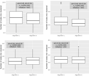
In this section we present the performance of the proposed algorithm on simulated datasets. The experiments cover three different scenarios: (1) dense network with communities of equal sizes; (2) dense network with communities of unequal sizes; and (3) sparse network. Recall the definition of ¯din (19). For each setting, we report results of Algorithm 1 initialized with four different approaches: USC(∞), USC(2 ¯d), NSC(0) and NSC( ¯d), the description of which can all be found in Section 2.3. For all these spectral clustering methods, Algorithm 2 was used to cluster the leading eigenvectors. The constantµin the critical radius definition was set to be 0.5 in all the results reported here. For each setting, the results are based on 100 independent draws from the underlying stochastic block model.
algorithm refines all the nodes with a single initialization on the whole network. Thus, the running time can be reduced roughly by a factor of n. Simulation results below suggest that the simplified version achieves similar performances to that of Algorithm 1 in all the settings we have considered. For the precise description of the simplified algorithm, we refer readers to Algorithm 3 in the appendix.
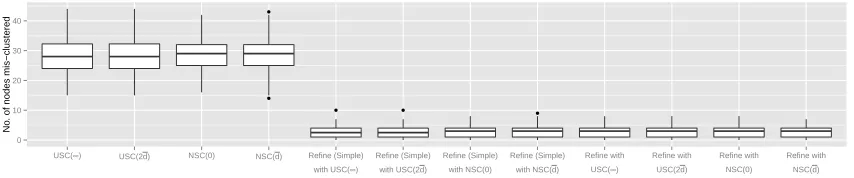
Balanced case In this setting, we generate networks with 2500 nodes and 10 communities, each of which consists of 250 nodes, and we set Bii = 0.48 for all i and Bij = 0.32 for
all i 6= j. Figure 1 shows the boxplots of the number of misclassified nodes. The first four boxplots correspond to the four different spectral clustering methods, in the order of USC(∞), USC(2 ¯d), NSC(0) and NSC( ¯d). The middle four correspond to the results achieved by applying the simplified refinement scheme with these four initialization methods, and the last four show the results of Algorithm 1 with these four initialization methods. Regardless of the initialization method, Algorithm 1 or its simplified version reduces the number of misclassified nodes from around 30 to around 5.
●
●
● ● ●
0 10 20 30 40
USC(∞) USC(2d) NSC(0) NSC(d) Refine (Simple) with USC(∞)
Refine (Simple) with USC(2d)
Refine (Simple) with NSC(0)
Refine (Simple) with NSC(d)
Refine with USC(∞)
Refine with USC(2d)
Refine with NSC(0)
Refine with NSC(d)
Refinement
No
. of nodes mis−clustered
Figure 1: Boxplots of number of misclassified nodes: Balanced case. Simple indicates that the simplified version of Algorithm 1 is used instead.
Imbalanced case In this setting, we generate networks with 2000 nodes and 4 commu-nities, the sizes of which are 200,400,600 and 800, respectively. The connectivity matrix is
B =
0.50 0.29 0.35 0.25 0.29 0.45 0.25 0.30 0.35 0.25 0.50 0.35 0.25 0.30 0.35 0.45
.
Hence, the within-community edge probability is no smaller than 0.45 while the between-community edge probability is no greater than 0.35, and the underlying SBM is inhomo-geneous. Figure 2 shows the boxplots of the number of misclassified nodes obtained by different initialization methods and their refinements, and the boxplots are presented in the same order as those in Figure 1. Similarly, we can see refinement significantly reduces the error.
● ●
●
● ● ●
● ●●●● ●●● ●●●●● ● ● ● ●●
0 5 10 15 20
USC(∞) USC(2d) NSC(0) NSC(d) Refine (Simple) with USC(∞)
Refine (Simple) with USC(2d)
Refine (Simple) with NSC(0)
Refine (Simple) with NSC(d)
Refine with USC(∞)
Refine with USC(2d)
Refine with NSC(0)
Refine with NSC(d)
Refinement
No
. of nodes mis−clustered
Figure 2: Boxplots of number of misclassified nodes: imbalanced case. Simple indicates that the simplified version of Algorithm 1 is used instead.
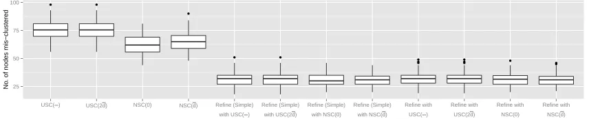
i6= j. The average degree of each node in the network is around 30. Figure 3 shows the boxplots of the number of misclassified nodes obtained by different initialization methods and their refinements, and the boxplots are presented in the same order as those in Figure 1. Compared with either USC or NSC initialization, refinement reduces the number of misclassified nodes by 50%.
● ●
●
● ●
● ●
● ●
●
● ●
● ●
25 50 75 100
USC(∞) USC(2d) NSC(0) NSC(d) Refine (Simple) with USC(∞)
Refine (Simple) with USC(2d)
Refine (Simple) with NSC(0)
Refine (Simple) with NSC(d)
Refine with USC(∞)
Refine with USC(2d)
Refine with NSC(0)
Refine with NSC(d)
Refinement
No
. of nodes mis−clustered
Figure 3: Boxplots of number of misclassified nodes: Sparse case. Simpleindicates that the simplified version of Algorithm 1 is used instead.
Summary In all three simulation settings, for all four initialization approaches consid-ered, the refinement scheme in Algorithm 1 (and its simplified version) was able to signifi-cantly reduce the number of misclassified nodes, which is in agreement with the theoretical properties presented in Section 3.
5. Discussion
In this section, we discuss a few important issues related to the methodology and the theory we have presented in the previous sections.
5.1 Error bounds when ab may not hold
Theorem 12 Suppose asn→ ∞, ak(a−logb)2k → ∞and Condition 1 is satisfied for γ satisfying
(16) andΘ = Θ0(n, k, a, b, β). Then for some positive constants c andC that depend only
on , for any sufficiently small constant 0 ∈ (0, c), if we replace the definition of tu’s in
(11) with
tu=
1 2log
bau(1−bbu/n) bbu(1−bau/n)
!
∧log 1
0/2
, (22)
then we have
sup (B,σ)∈Θ
PB,σ
`(σ,σb)≥exp
−(1−C0) nI∗
2
→0, if k= 2,
sup (B,σ)∈Θ
PB,σ
`(σ,σb)≥exp
−(1−C0) nI∗
βk
→0, if k≥3,
(23)
whereI∗is defined as in (14). In particular, we can setC = 103 2− 2log
2
andc = min(101C,2−).
If in addition Condition 1 is satisfied for γ satisfying both (16) and (18) and Θ = Θ(n, k, a, b, λ, β;α), then the same conclusion holds for Θ = Θ(n, k, a, b, λ, β;α).
Compared with the conclusion (17) in Theorem 4, the vanish sequence η in the ex-ponent of the upper bound is replaced by C0, which is guaranteed to be smaller than min(0.1,log(22/)) and can be driven to be arbitrarily small by decreasing0. To achieve this, thetu’s used in defining the penalty parameters in the penalized neighbor voting step need
to be truncated at the value log0/12. 5.2 Implications of the results
We now discuss some implications of the results in Theorems 4 – 12.
When using USC as initialization for Algorithm 1, we obtain the following results by combining Theorem 4, Theorem 6 and Theorem 12. Recall that ¯d is the average degree of nodes inA defined in (19).
Theorem 13 Consider Algorithm 1 initialized by σ0 with USC(τ) with τ =Cd¯for some sufficiently large constant C >0. If as n→ ∞, ab and
(a−b)2
ak3logk → ∞, (24)
then there is a sequenceη →0 such that (17)holds withΘ = Θ0(n, k, a, b, β). If asn→ ∞, ab and
λ2
ak(logk+a/(a−b)) → ∞, (25)
then (17) holds forΘ = Θ(n, k, a, b, λ, β;α). If for either parameter space, a b may not hold but k is fixed and (24) or (25) holds respectively, then (23) holds as long as tu is
Compared with Theorem 1, the minimax optimal performance is achieved under mild conditions. Take Θ = Θ0(n, k, a, b, β) for example. For any fixed k, the minimax optimal misclassification proportion is achieved with high probability only under the additional condition ofab. In addition, weak consistency is achieved for fixedkas long as (a−ab)2 → ∞, regardless of the behavior of ab. This condition is indeed necessary and sufficient for weak consistency. See, for instance, Mossel et al. (2012, 2013b); Yun and Proutiere (2014b); Zhang and Zhou (2015). To achieve strong consistency for fixedk, it suffices to ensure`(σ,bσ)<
1
n
and Theorem 13 implies that it is sufficient to have
lim inf
n→∞
nI∗
2 logn >1, whenk= 2; lim infn→∞
nI∗
βklogn >1, when k≥3, (26)
regardless of the behavior of ab. On the other hand, Theorem 1 shows that it is impossible to achieve strong consistency if
lim sup
n→∞
nI∗
2 logn <1, whenk= 2; lim supn→∞
nI∗
βklogn <1, when k≥3. (27)
When an = o(1), nI∗ = (1 +o(1))(√a−√b)2 and so one can replace nI∗ in (26) – (27) with (√a−√b)2. In the literature, Abbe et al. (2014) and Mossel et al. (2014) obtained comparable strong consistency results via efficient algorithms for the special case of two communities of equal sizes, i.e., k = 2 andβ = 1. Abbe and Sandon (2015a) investigated the case of fixedkandβ ≥1. Their results give necessary and sufficient conditions for each instance of model parameters. In comparison, our result characterizes minimax optimality through worst case analysis and is less general than those of Abbe and Sandon (2015a). On the other hand, compared with Abbe and Sandon (2015a), we allow any fixed k and any β ≥ 1 without assuming a b logn. In the weak consistency regime, in terms of misclassification proportion, for the special case of k = 2 and β = 1, Yun and Proutiere (2014a) achieved the optimal rate for Θ0(n,2, a, b,1) when a b a−b, while the error bounds in other papers are typically off by a constant multiplier on the exponent. In comparison, Theorem 13 provides optimal results (17) and near optimal results (23) for a much broader class of models under much weaker conditions. Last but not least, our algorithm can provably achieve strong consistency and minimax optimal performance even for growingk, which to our limited knowledge, is the first in the literature.
The performance of Algorithm 1 initialized by NSC can be summarized as the following theorem by combining Theorem 4, Theorem 10 and Theorem 12. In this case, the sufficient condition for achieving minimax optimal performance is slightly stronger than when USC is used for initialization.
Theorem 14 Consider Algorithm 1 initialized by σ0 with NSC(τ) with τ =Cd¯for some
sufficiently large constant C >0. If as n→ ∞, ab and
(a−b)2
ak3logkloga → ∞, (28)
then there is a sequenceη →0 such that (17)holds withΘ = Θ0(n, k, a, b, β). If asn→ ∞, ab and
λ2
then (17) holds forΘ = Θ(n, k, a, b, λ, β;α). If for either parameter space, a b may not hold but k is fixed and (28) or (29) holds respectively, then (23) holds as long as tu is
replaced by (22) in Algorithm 1.
Last but not least, we would like to point out that when the key parameters a and b
are known, we can obtain the desired performance guarantee under weaker conditions as summarized in the following theorem.
Theorem 15 (The case of known a, b) Suppose a, b are known. Consider Algorithm 1 initialized by σ0 with USC(τ) with τ =Ca for some sufficiently large constant C > 0 and
b
au=a,bbu =b in (9) for all u∈[n]. If asn→ ∞, ab and
(a−b)2
ak3 → ∞, (30)
then there is a sequenceη →0 such that (17)holds withΘ = Θ0(n, k, a, b, β). If asn→ ∞, ab and
λ2
ak → ∞, (31)
then(17)holds withΘ = Θ(n, k, a, b, λ, β;α). If for either parameter space without assuming
ab, (30) or (31) holds respectively, then (23) holds if in addition tu is replaced by (22).
If instead NSC(τ) is used for initialization with τ = Ca for some sufficiently large constant C >0, then the above conclusions hold if we replace (30) with ak(a3−logb)2a → ∞ and
(31) with akλlog2 a → ∞, respectively.
6. Proofs of main results
The main result of the paper, Theorem 4, is proved in Section 6.1. Theorem 6 and Theorem 10 are proved in Section 6.2 and Section 6.3 respectively. The proofs of the remaining results, together with some auxiliary lemmas, are given in the appendix.
6.1 Proof of Theorem 4
We first state a lemma that guarantees the accuracy of parameter estimation in Algorithm 1.
Lemma 16 Let Θ = Θ(n, k, a, b, λ, β;α). Suppose as n→ ∞, (a−akb)2 → ∞ and Condition 1 holds with γ satisfying (16) and (18). Then there is a sequence η→ 0 as n→ ∞ and a constant C >0 such that
min
u∈[n](B,σinf)∈ΘP
min
π∈Sk
max
i,j∈[k]|
b
Buij−Bπ(i)π(j)| ≤η
a−b n
≥1−Cn−(1+δ). (32)
Proof 1◦ Let Θ = Θ(n, k, a, b, λ, β;α). For any community assignments σ1 andσ2, define
`0(σ1, σ2) = 1
n
n X
u=1
1{σ1(u)6=σ2(u)}. (33)
Fix any (B, σ)∈Θ andu∈[n]. Define event
Eu=
`0(πu(σ), σu0)≤γ . (34)
To simplify notation, assume thatπu = Id is the identity permutation.
Fix any i∈[k]. OnEu,
ni ≥ |Ceiu∩ Ci| ≥ni−γ1n, |Ceiu∩ Cic| ≤γ2n, where γ1, γ2 ≥0 andγ1+γ2 ≤γ. (35)
Let C0i be any deterministic subset of [n] such that (35) holds with Ceiu replaced by Ci0. By
definition, there are at most
γn X l=0 ni l γn X m=0
n−ni
m
≤(γn+ 1)2
eni γn γn en γn γn ≤exp
2 log(γn+ 1) + 2γnloge
γ
≤exp
C1γnlog 1
γ
different subsets with this property where C1 > 0 is an absolute constant. Let Ei0 be the
edges withinCi0. Then|Ei0|consists of independent Bernoulli random variables, where at least (1−βγk)2 proportion of them follow the Bern(Bii) distribution, at most (βγk)2 proportion
that are stochastically smaller than Bern(αan ) and stochastically larger than Bern(na), and at most 2βγk proportion are stochastically smaller than Bern(nb). Therefore, we obtain that
(1−βγk)2Bii+ (βγk)2
a n ≤E
"
|Ei0|
1 2|C
0
i|(|Ci0| −1) #
≤ max
t∈[0,βγk]
(1−t)2Bii+t2
αa n + 2t
b n
.
(36)
Note that the LHS is (1−(2 +o(1))βγk)Bii. On the other hand, under condition (18), the
RHS is attained at t= 0 and equals Bii exactly. Thus, we conclude that
E "
|Ei0|
1 2|C
0
i|(|Ci0| −1) #
−Bii
≤Cβγkαa n =η
0
a−b n
(37)
for some η0 → 0 that depends only ona, k, α, β and γ, where the last inequality is due to (18).
On the other hand, by Bernstein’s inequality, for anyt >0,
P|Ei0| −E|Ei0|
> t ≤2 exp (
− t
2
2(12(ni+γn)2αan +23t) )
Let
t2 = (ni+γn)2
αa
n (C1γnlogγ
−1+ (3 +δ) logn)∨(2C
1γnlogγ−1+ 2(3 +δ) logn)2
.n
k
p
aγlogγ−1+γnlogγ−12,
where we the second inequality holds since logxx is monotone decreasing asx increases and soγlogγ−1 ≥ 1
nlognfor anyγ ≥
1
n, which is the case of most interest sinceγ <
1
n leads to
γ = 0 and so the initialization is already perfect. Even when γ = 0, we can still continue to the following arguments by replacing every γ with 1n and all the steps continue to hold. Thus, we obtain that for positive constantCα,β,δ that depends only onα, β and δ,
P n
|Ei0| −E|Ei0|
> Cα,β,δ n
k
p
aγlogγ−1+γnlogγ−1o≤exp
−C1γnlogγ−1 n−(3+δ). (38)
Thus, with probability at least 1−exp
−C1γnlogγ−1 n−(3+δ),
|E0 i| 1 2|C 0 i|(|C
0 i| −1)
−E |E
0 i|
1 2|C
0 i|(|C
0 i| −1)
≤Cα,β,δ
k n
p
aγlogγ−1+k
2γlogγ−1 n
=η0
a−b n
,
(39)
whereη0 →0 depends only ona, k, α, β, γ and δ. Here, the last inequality holds since
kpaγlogγ−1 =√akpkγlogγ−1, where√aka−bsince (aak−b)2 → ∞and kγlogγ−1 =O(1), and
k2γlogγ−1 =kγlogγ−1·k.k (a−b)
2
a .a−b.
We combine (37) and (39) and apply the union bound to obtain that for a sequence η→0 that depends only ona, k, α, β, γ andδ, with probability at least 1−n−(3+δ)
|Eeiu|
1
2|Ceiu|(|Ceiu| −1)
−Bii ≤η
a−b n
. (40)
The proof for Bij estimation is analogous and hence is omitted. A final union bound on
i, j ∈ [k] leads to the desired claim since all the constants and vanishing sequences in the above analysis depend only ona, b, k, α, β, γ and δ, but not onu,B orσ.
2◦ If Θ = Θ0(n, k, a, b, β), then condition (18) onγ is no longer needed. This is because (36) can be replaced by
min
t∈[0,βγk]
(1−t)2a
n+ 2t(1−t) b n +t
2b n ≤E " |E0 i| 1 2|C 0
i|(|Ci0| −1) #
≤ max
t∈[0,βγk]
(1−t)2a
n +t 2a
n+ 2t(1−t) b n
where the LHS equals an −(1−βγk(1 +o(1)))a−nb = na +o(a−nb) and the RHS equals an. Thus, no additional condition is needed to guarantee (37) in the foregoing arguments. This completes the proof.
The next two lemmas establish the desired error bound for the node-wise refinement.
Lemma 17 Let Θ0 be defined as in (2) and k ≥2. Suppose as n→ ∞, (a
−b)2
ak → ∞ and
a b. If there exists two sequences γ = o(1/k) and η = o(1), constants C, δ > 0 and permutations{πu}nu=1⊂Sk such that
inf (B,σ)∈Θ0
min
u∈[n]P
n
`0(πu(σ), σu0)≤γ, |bau−a| ≤η(a−b), |bbu−b| ≤η(a−b) o
≥1−Cn−(1+δ).
(41)
Then for bσu(u) defined as in (10) with ρ =ρu in (12), there is a sequence η0 =o(1) such
that for k= 2,
sup (B,σ)∈Θ0
max
u∈[n]P
{σbu(u)6=πu(σ(u))} ≤(k−1) exp
−(1−η0)nI
∗
2
+Cn−(1+δ),
and for k≥3,
sup (B,σ)∈Θ0
max
u∈[n]P
{σbu(u)6=πu(σ(u))} ≤(k−1) exp
−(1−η0)nI
∗
βk
+Cn−(1+δ). Proof In what follows, letEu denote the event in (41). For the sake of brevity, we letp=
a/n,q =b/n,pbu =abu/n and qbu =bbu/n. Moreover, letσu =πu(σ), ni =|{v:σu(v) =i}|,
mi =|{v:σ0u(v) = i}| and m0i =|{v :σ0u(v) = σu(v) = i}|. Without loss of generality, let
σu(u) = 1.
Then we have
P{bσu(u)6= 1 and Eu} ≤ X
l6=1
P
Eu and X
σu(v)=l
Auv− X
σu(v)=1
Auv≥ρu(ml−m1)
=X
l6=1 pl.
(42)
Now we bound each pl. By the independence structure and Chernoff bound, we have
pl ≤ E n
exp (−tuρu(ml−m1)) (qetu+ 1−q)m
0
l(petu+ 1−p)ml−m0l
(pe−tu+ 1−p)m01(qe−tu+ 1−q)m1−m011 {Eu}
o
(43)
≤ E
exp (−tuρu(ml−m1)) (qetu+ 1−q)ml(pe−tu+ 1−p)m11{Eu} (44)
×E
(
petu+ 1−p
qetu+ 1−q
ml−m0l
qe−tu+ 1−q
pe−tu+ 1−p
m1−m01
1{Eu} )
. (45)
We are going to give bounds for the terms in (44) and (45) respectively. Before doing that, we need some preparatory inequalities. Definet∗ through the equation
et∗ =
s
p(1−q)
Then, on the eventEu,
etu−t∗+et∗−tu ≤exp(C
1η), (46)
for some constantC1>0. Moreover,
|etu−1| ∨ |e−tu−1| ≤C
2 p−q
p =C2 a−b
a , (47)
for some constantC2>0. Therefore, for the term in (44), on the eventEu,
exp (−tuρu(ml−m1)) (qetu+ 1−q)ml(pe−tu+ 1−p)m1 = exp (−tuρu(ml−m1)) qetu+ 1−q
(ml−m1)/2
pe−tu+ 1−p(m1−ml)/2
(48)
× qetu+ 1−q(m1+ml)/2
pe−tu+ 1−p(m1+ml)/2
. (49)
By (46), the term in (49) is upper bounded by
pq+ (1−p)(1−q) +√pqp(1−p)(1−q)(etu−t∗+et∗−tu) m1+ml
2
≤exp
−(1 +o(1))m1+ml
2 I
∗
≤exp
−(1 +o(1))n1+nl
2 I
∗
.
By (47), the term in (48) is upper bounded by
exp (−tuρu(ml−m1)) qetu+ 1−q
(ml−m1)/2
pe−tu+ 1−p(m1−ml)/2
= exp
m1−ml
2
logpe
−tu+ 1−p
qetu+ 1−q −log b
pue−tu+ 1−pbu
b
quetu+ 1−qbu
≤ exp
|m1−ml|
2 |e
−tu−1||
b
pu−p|+|etu−1||qbu−q| ≤ exp o n k
(p−q)2
p
= exp
o(1)n1+nl
2 I
∗
.
Therefore, we can upper bound (44) as
E n
e−tuρu(ml−m1)(qetu+ 1−q)ml(pe−tu+ 1−p)m11 {Eu}
o
≤exp
−(1 +o(1))n1+nl
2 I
∗
.
(50) Now we provide an upper bound for (45). By (47), onEu,
petu+ 1−p
qetu+ 1−q = 1 +
(p−q)(etu−1)
qetu+ 1−q ≤1 +O
(p−q)2
p ≤exp O
(p−q)2
p
,
and
qe−tu+ 1−q
pe−tu+ 1−p = 1 +
(p−q)(1−e−tu)
pe−tu+ 1−p ≤1 +O
(p−q)2
p ≤exp O
(p−q)2
p
Therefore,
E (
petu+ 1−p
qetu+ 1−q
ml−m0l
qe−tu+ 1−q
pe−tu+ 1−p
m1−m01
1{Eu} )
≤exp
o(1)n1+nl
2 I
∗
. (51)
By combining (50) and (51), we have
pl≤exp
−(1 +o(1))n1+nl
2 I
∗
. (52)
Using (42), this implies
P{bσu(u)6= 1 and Eu} ≤(k−1) exp
−(1 +o(1)) min
l6=1
n1+nl
2 I∗ , and so
P{σbu(u)6= 1} ≤(k−1) exp
−(1 +o(1)) min
l6=1
n1+nl
2
I∗
+Cn−(1+δ).
When k= 2, minl6=1 n1+2nl
= n2, and when k≥3, minl6=1 n1+2nl
≥ βkn. Thus, the proof is complete.
Lemma 18 Let Θ be defined as in (3) and k ≥ 2. Suppose as n → ∞, (a−akb)2 → ∞ and
a b. If there exists two sequences γ = o aak−b
and η = o(1), constants C, δ > 0 and permutations {πu}nu=1 ⊂ Sk such that (41) holds. Then for bσu(u) defined as in (10) with
ρ=ρu in (12), the conclusions of Lemma 17 continue to hold.
Proof The proof is similar to that of Lemma 17 and we use the same notation as there. First, we give a bound for pl defined in (42). Let Xj ∼ Bern(q), Yj ∼Bern(p) and Zj ∼
Bern(αp), j≥1, be mutually independent. Then, a stochastic order argument gives
pl ≤ E
P
m0l X
j=1 Xj+
ml−m0l X
j=1 Zj−
m0
1 X
j=1
Yj ≥ρ(ml−m1) and Eu A−u
≤ Eexp (−tuρu(ml−m1)) (qetu+ 1−q)ml(pe−tu+ 1−p)m11{Eu} (53)
×E (
1
qetu+ 1−q
ml−m0l 1
pe−tu+ 1−p
m1−m01
(54)
(αpetu+ 1−αp)ml−m0l1{ Eu}
o
.
Note that the term in (53) is the same as that in (44), and thus it can be upper bounded by (50) as before. To bound for (54), observe that by (47),
1
qetu+ 1−q ≤exp q|e
1
pe−tu+ 1−p ≤exp Cp|e
−tu−1|
≤exp (O(p−q))
and
αpetu+ 1−αp≤exp αp|etu−1|
≤exp (O(p−q)).
Thus, under the assumptionγ =o
p−q
kp
, the term (54) is bounded by exp o(1)n1+nl
2 I
∗
. The remaining proof is the same as that of Lemma 17.
Finally, we need a lemma to justify the consensus step in Algorithm 1.
Lemma 19 For any community assignments σ and σ0: [n] → [k], such that for some constant C ≥1
min
l∈[k]
| {u:σ(u) =l} |,min
l∈[k]
|
u:σ0(u) =l | ≥ n
Ck, and πmin∈Sk
`0(σ, π(σ0))< 1
Ck.
Define map ξ: [k]→[k] as
ξ(i) = argmax
l
{u:σ(u) =l} ∩ {u:σ0(u) =i}
, ∀i∈[k]. (55)
Then ξ∈Sk and `0(σ, ξ(σ0)) = minπ∈Sk`0(σ, π(σ 0)).
Proof By the definition in (55), we obtain
ξ = argmin
ξ0:[k]→[k]
`0(σ, ξ0(σ0)), and `0(σ, ξ(σ0))≤ min
π∈Sk
`0(σ, π(σ0))< 1
Ck.
Thus, what remains to be shown is that ξ ∈Sk, i.e., ξ(l1) =6 ξ(l2) for any l1 6=l2. To this end, note that if for some l1 6=l2, ξ(l1) =ξ(l2), then there would exist some l0 ∈[k] such that for anyl∈[k], ξ(l)6=l0, and so
`0(σ, ξ(σ0))≥ 1
n
X
u:σ(u)=l0
1{σ(u)6=ξ(σ0(u))}=
| {u:σ(u) =l0} |
n ≥
1
Ck.
This is in contradiction to the second last display, and hence ξ ∈ Sk. This completes the
proof.
Proof [Proof of Theorem 4] Let Θ = Θ(n, k, a, b, λ, β;α), and fix any (B, σ)∈Θ. For any
u∈[n], by Condition 1 and the fact thatσ0uandbσu differ only at the community assignment
of u, forγ0 =γ+ 1/n, there exists someπu ∈Sk such that
P`0(σ, π−u1(bσu))≤γ 0
n ≥1−C0n−(1+δ). (56)
Without loss of generality, we assume π1 = Id is the identity map. Now for any fixed u ∈ {2, . . . , n}, define map ξu : [k]→ [k] as in (55) with σ and σ0 replaced by bσ1 and bσu.
Then by definition
b
In addition, (56) implies with probability at least 1−Cn−(1+δ), we have
`0(σ,bσ1)≤γ 0
and `0(σ, π−u1(bσu))≤γ 0
.
So the triangle inequality implies `0(bσ1, π
−1
u (bσu))≤2γ
0 and hence the condition of Lemma
19 is satisfied. Thus, Lemma 19 implies
Pξu=π−u1 ≥1−Cn
−(1+δ). (58)
Whenk≥3, Lemma 16, (16) and (18) imply that the condition of Lemma 18 is satisfied, which in turn implies that for a sequence η0=o(1),
P{bσ(u)6=σ(u)}=P{ξu(σbu(u))6=σ(u)}
≤P
ξu(bσu(u))6=σ(u), ξu=π
−1
u +P
ξu6=π−u1
≤P{bσu(u)=6 πu(σ(u))}+P
ξu 6=πu−1
≤Cn−(1+δ)+ (k−1) exp
−(1−η0)nI
∗
βk
.
Set
η=η0+β
r
k
nI∗ =o(1) (59)
where the last inequality holds since nIk∗ (a−akb)2 → ∞. Thus, Markov’s inequality leads to
P
`0(σ,bσ)>(k−1) exp
−(1−η)nI
∗
βk
≤ 1
(k−1) exp
n
−(1−η)nIβk∗
o 1 n n X u=1
P{σb(u)6=σ(u)}
≤exp
−(η−η0)nI
∗
βk
+ Cn
−(1+δ)
(k−1) exp
n
−(1−η)nIβk∗
o ≤exp ( − r nI∗ k ) + Cn
−(1+δ)
(k−1) exp
n
−(1−η)nIβk∗
o.
If (k−1) exp
n
−(1−η)nIβk∗
o
≥n−(1+δ/2), then
P
`0(σ,bσ)>(k−1) exp
−(1−η)nI
∗ βk ≤exp ( − r nI∗ k )
+Cn−δ/2 =o(1).
If (k−1) expn−(1−η)nIβk∗o< n−(1+δ/2), then
P
`0(σ,σb)>(k−1) exp
−(1−η)nI
∗
βk
=P{`0(σ,σb)>0} ≤ n X
u=1
P{bσ(u)6=σ(u)}
≤n(k−1) exp
−(1−η)nI
∗
βk
Here, the second last inequality holds sinceη > η0 and so (k−1) exp{−(1−η0)nI∗/(βk)}<
(k−1) exp{−(1−η)nI∗/(βk)}< n−(1+δ/2). We complete the proof for the case of Θ(n, k, a, b, λ, β;α) and k≥3 by noting that (k−1) expn−(1−η)nIβk∗o= expn−(1−η00)nIβk∗ofor another
se-quence η00 =o(1) under the assumption ak(a−logb)2k → ∞ and no constant or sequence in the foregoing arguments involves B, σ or u. When Θ = Θ(n, k, a, b, λ, β;α) and k = 2, the foregoing arguments continue to hold withβ and kreplaced with 1 and 2 respectively.
When Θ = Θ0(n, k, a, b, β), we can run the foregoing arguments with Lemma 18 replaced by Lemma 17 to reach the conclusion in (17), which does not require condition (18). This completes the proof.
6.2 Proof of Theorem 6
The following lemma is critical to establish the result of Theorem 6. Its proof is given in the appendix. Let us introduce the notation O(k1, k2) = {V ∈ Rk1×k2 : VTV = Ik2} for
k1≥k2.
Lemma 20 Consider a symmetric adjacency matrixA∈ {0,1}n×nand a symmetric matrix
P ∈[0,1]n×n satisfyingAuu= 0 for allu∈[n]and Auv∼Bernoulli(Puv) independently for
allu > v. For any C0 >0, there exists some C >0 such that
kTτ(A)−Pkop≤C
p
npmax+ 1,
with probability at least1−n−C0 uniformly overτ ∈[C1(npmax+ 1), C2(npmax+ 1)] for some
sufficiently large constants C1, C2, where pmax= maxu≥vPuv.
Lemma 21 ForP = (Puv) = (Bσ(u)σ(v)), we have SVD P =UΛUT, where U =Z∆−1W,
with ∆ =diag(√n1, ...,
√
nk), Z ∈ {0,1}n×k is a matrix with exactly one nonzero entry in
each row at (i, σ(i))taking value 1 andW ∈O(k, k).
Proof Note that
P =ZBZT =Z∆−1∆B∆(Z∆−1)T,
and observe that Z∆−1 ∈O(n, k). Apply SVD to the matrix ∆B∆T =WΛWT for some
W ∈O(k, k), and then we have P =UΛUT withU =Z∆−1W ∈O(k, k).
Proof [Proof of Theorem 6] Under the current assumption,Eτ ∈[C10a, C20a] for some large C10 and C20. Using Bernstein’s inequality, we have τ ∈[C1a, C2a] for some large C1 and C2 with probability at least 1−e−C0n. When (20) holds, by Lemma 20, we deduce that thekth
eigenvalue of Tτ(A) is lower bounded by c1λk with probability at least 1−n−C
0
we have kUb −U W1kF ≤ C √
k
λkkTτ(A)−Pkop for some W1 ∈ O(k, k) and some constant
C >0. Applying Lemma 21, we have
kUb−VkF ≤C
√
k λk
kTτ(A)−Pkop, (60)
whereV =Z∆−1W2 ∈O(n, k) for someW2 ∈O(k, k). Combining (60), Lemma 20 and the conclusionτ ∈[C1a, C2a], we have
kUb−VkF≤
C√k√a λk
, (61)
with probability at least 1−n−C0. The definition of V implies that
kVu∗−Vv∗k= r
1
nu
+ 1
nv
1{σ(u)6=σ(v)}. (62)
In other words, define Q = ∆−1W2 ∈ Rk×k and we have Vu∗ = Qσ(u)∗ for each u ∈ [n].
Hence, for σ(u) 6= σ(v), Qσ(u)∗−Qσ(v)∗
= kVu∗−Vv∗k ≥ q
2k
βn. Recall the definition
r=µ
q k
n in Algorithm 2. Define the sets
Ti = n
u∈σ−1(i) :
Ubu∗−Qi∗ < r 2 o
, i∈[k].
By definition, Ti∩Tj =∅when i6=j, and we also have
∪i∈[k]Ti = n
u∈[n] :
Ubu∗−Vu∗ < r 2 o . (63) Therefore,
∪i∈[k]Ti c
r2
4 ≤
X
u∈[n]
Ubu∗−Vu∗ 2 ≤ C 2ka λ2k ,
where the last inequality is by (61). After rearrangement, we have
∪i∈[k]Tic≤
4C2na µ2λ2
k
. (64)
In other words, most nodes are close to the centers and are in the set (63). Note that the sets {Ti}i∈[k] are disjoint. Suppose there is somei∈[k] such that|Ti|<|σ−1(i)| −
∪i∈[k]Ti c
,
we have∪i∈[k]Ti =
P
i∈[k]|Ti|< n−
∪i∈[k]Ti c
=
∪i∈[k]Ti
, which is impossible. Thus,
the cardinality of Ti for each i∈[k] is lower bounded as
|Ti| ≥ |σ−1(i)| −
∪i∈[k]Ti c
≥
n βk −
4C2na µ2λ2
k
> n
2βk, (65)
![Figure 4: The schematic plot for the proof of Theorem 6. The balls {Ti}i∈[k] are centered at {Qi}i∈[k],and the centers are at least�2kβ n away from each other](https://thumb-us.123doks.com/thumbv2/123dok_us/9785242.1964017/29.612.133.479.89.306/figure-schematic-plot-proof-theorem-balls-centered-centers.webp)