Approximation Vector Machines for Large-scale Online Learning

(1)

Approximation Vector Machines

for Large-scale Online Learning

Trung Le [email protected]

Tu Dinh Nguyen [email protected]

Vu Nguyen [email protected]

Dinh Phung [email protected]

Centre for Pattern Recognition and Data Analytics, School of Information Technology,

Deakin University, Australia, Waurn Ponds Campus

Editor:Koby Crammer

Abstract

One of the most challenging problems in kernel online learning is to bound the model size and to promote model sparsity. Sparse models not only improve computation and memory usage, but also enhance the generalization capacity – a principle that concurs with the law of parsimony. However, inappropriate sparsity modeling may also significantly degrade the performance. In this paper, we propose Approximation Vector Machine (AVM), a model that can simultaneously encourage sparsity and safeguard its risk in compromising the per-formance. In an online setting context, when an incoming instance arrives, we approximate this instance by one of its neighbors whose distance to it is less than a predefined threshold. Our key intuition is that since the newly seen instance is expressed by its nearby neigh-bor the optimal performance can be analytically formulated and maintained. We develop theoretical foundations to support this intuition and further establish an analysis for the common loss functions including Hinge, smooth Hinge, and Logistic (i.e., for the classifi-cation task) and`1, `2, andε-insensitive (i.e., for the regression task) to characterize the gap between the approximation and optimal solutions. This gap crucially depends on two key factors including the frequency of approximation (i.e., how frequent the approximation operation takes place) and the predefined threshold. We conducted extensive experiments for classification and regression tasks in batch and online modes using several benchmark datasets. The quantitative results show that our proposed AVM obtained comparable pre-dictive performances with current state-of-the-art methods while simultaneously achieving significant computational speed-up due to the ability of the proposed AVM in maintaining the model size.

Keywords: kernel, online learning, large-scale machine learning, sparsity, big data, core set, stochastic gradient descent, convergence analysis

1. Introduction

In modern machine learning systems, data usually arrive continuously in stream. To enable efficient computation and to effectively handle memory resource, the system should be able to adapt according to incoming data. Online learning represents a family of efficient and scalable learning algorithms for building a predictive model incrementally from a sequence

c

(2)

of data examples (Rosenblatt, 1958; Zinkevich, 2003). In contrast to the conventional learning algorithms (Joachims, 1999; Chang and Lin, 2011), which usually require a costly procedure to retrain the entire dataset when a new instance arrives, online learning aims to utilize the new incoming instances to improve the model given the knowledge of the correct answers to previous processed data (and possibly additional available information), making them suitable for large-scale online applications wherein data usually arrive sequentially and evolve rapidly.

The seminal line of work in online learning, referred to as linear online learning

(Rosen-blatt, 1958; Crammer et al., 2006; Dredze et al., 2008), aims at learning a linear predictor in the input space. The crucial limitation of this approach lies in its over-simplified linear modeling choice and consequently may fail to capture non-linearity commonly seen in many

real-world applications. This motivated the works in kernel-based online learning (Freund

and Schapire, 1999; Kivinen et al., 2004) in which a linear model in the feature space corre-sponding with a nonlinear model in the input space, hence allows one to cope with a variety of data distributions.

One common issue with kernel-based online learning approach, also known as the curse

of kernelization, is that the model size (i.e., the number of vectors with non-zero coefficients) may grow linearly with the data size accumulated over time, hence causing computational problem and potential memory overflow (Steinwart, 2003; Wang et al., 2012). Therefore in practice, one might prefer kernel-based online learning methods with guaranty on a limited and bounded model size. In addition, enhancing model sparsity is also of great interest to practitioners since this allows the generalization capacity to be improved; and in many cases leading to a faster computation. However, encouraging sparsity needs to be done with care since an inappropriate sparsity-encouraging mechanism may compromise the performance. To address the curse of kernelization, budgeted approaches (Crammer et al., 2004; Dekel et al., 2005; Cavallanti et al., 2007; Wang and Vucetic, 2010; Wang et al.,

2012; Le et al., 2016a,c) limits the model size to a predefined budgetB. Specifically, when

the current model size exceeds this budget, a budget maintenance strategy (e.g., removal,

projection, or merging) is triggered to recover the model size back to the budgetB. In these

approaches, determining a suitable value for the predefined budget in a principled way is important, but challenging, since setting a small budget makes the learning faster but may suffer from underfitting, whereas a large budget makes the model fit better to data but may dramatically slow down the training process. An alternative way to address the curse of kernelization is to use random features (Rahimi and Recht, 2007) to approximate a kernel function (Ming et al., 2014; Lu et al., 2015; Le et al., 2016b). For example, Lu et al. (2015) proposed to transform data from the input space to the random-feature space, and then performed SGD in the feature space. However, in order for this approach to achieve good kernel approximation, excessive number of random features is required which could lead to a serious computational issue. To reduce the impact number of random features, Le et al. (2016b) proposed to distribute the model in dual space including the original feature space and the random feature space that approximates the first space.

(3)

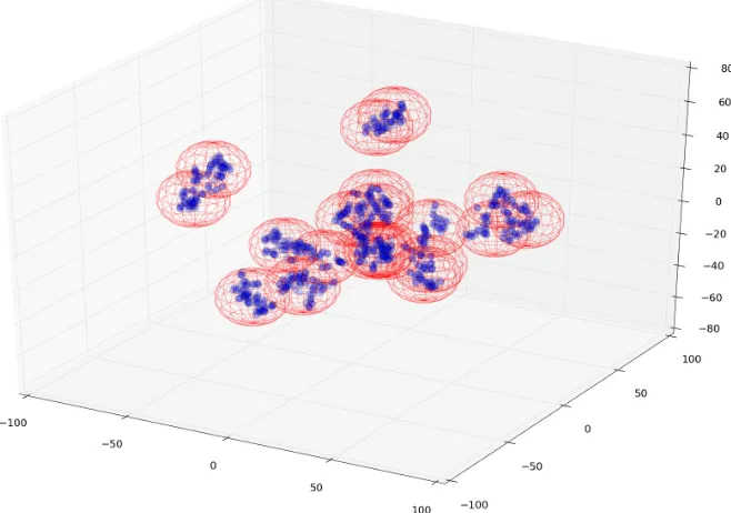
Figure 1: An illustration of the hypersphere coverage for 1,000 data samples which locate in

3D space. We cover this dataset using hyperspheres with the diameterδ= 7.0, resulting in

20 hypersphere cells as shown in the figure (cf. Sections (6.3,9)). All data samples in a same cell are approximated by a core point in this cell. The model size is therefore significantly

reduced from 1,000 to 20.1

In this paper, we propose Approximation Vector Machine (AVM) to simultaneously

encourage model sparsity2 _{while preserving the model performance.} _{Our model size is}

theoretically proven to be bounded regardless of the data distribution and data arrival

order. To promote sparsity, we introduce the notion ofδ-coverage which partitions the data

space into overlapped cells whose diameters are defined byδ (cf. Figure 1). This coverage

can be constructed in advance or on the fly. Our experiment on the real datasets shows

that the coverage can impressively boost sparsity; for example with datasetKDDCup99 of

4,408,589 instances, our model size is 115 withδ= 3 (i.e., only 115 cells are required); with

datasetairlines of 5,336,471 instances, our model size is 388 with δ= 1.

In an online setting context, when an incoming instance arrives, it can be approximated with the corresponding core point in the cell that contains it. Our intuitive reason is that when an instance is approximated by an its nearby core point, the performance would be largely preserved. We further developed rigorous theory to support this intuitive reason. In particular, our convergence analysis (covers six popular loss functions, namely Hinge,

smooth Hinge, and Logistic for classification task and`2,`1, andε-insensitive for regression

task) explicitly characterizes the gap between the approximate and optimal solutions. The analysis shows that this gap crucially depends on two key factors including the cell diameter

(4)

δand the approximation process. In addition, the cell parameterδcan be used to efficiently control the trade-off between sparsity level and the model performance. We conducted ex-tensive experiments to validate the proposed method on a variety of learning tasks, including classification in batch mode, classification and regression in online mode on several bench-mark large-scale datasets. The experimental results demonstrate that our proposed method maintains a comparable predictive performance while simultaneously achieving an order of magnitude speed-up in computation comparing with the baselines due to its capacity in maintaining model size. We would like to emphasize at the outset that unlike budgeted algorithms (e.g., (Crammer et al., 2004; Dekel et al., 2005; Cavallanti et al., 2007; Wang and Vucetic, 2010; Wang et al., 2012; Le et al., 2016a,c, 2017)), our proposed method is nonparametric in the sense that the number of core sets grow with data on demand, hence care should be exercised in practical implementation.

The rest of this paper is organized as follows. In Section 2, we review works mostly related to ours. In Section 3, we present the primal and dual forms of Support Vector Machine (SVM) as they are important background for our work. Section 4 formulates the proposed problem. In Section 5, we discuss the standard SGD for kernel online learning

with an emphasis on thecurse of kernelization. Section 6 presents our proposed AVM with

full technical details. Section 7 devotes to study the suitability of loss functions followed by Section 8 where we extend the framework to multi-class setting. Finally, in Section 9, we conduct extensive experiments on several benchmark datasets and then discuss experimental results as well as their implications. In addition, all supporting proof is provided in the appendix sections.

2. Related Work

One common goal of online kernel learning is to bound the model size and to encourage sparsity. Generally, research in this direction can be broadly reviewed into the following themes.

Budgeted Online Learning. This approach limits the model size to a predefined budget

B. When the model size exceeds the budget, a budget maintenance strategy is triggered

to decrement the model size by one. Three popular budget maintenance strategies are

(5)

projection onto the linear span of others in the feature space exceeds a predefined threshold, or otherwise its information is kept through the projection. Other works involving the pro-jection strategy include Budgeted Passive Aggressive Nearest Neighbor (BPA-NN) (Wang and Vucetic, 2010; Wang et al., 2012). The merging strategy was used in some works (Wang and Vucetic, 2009; Wang et al., 2012).

Random Features. The idea of random features was proposed in (Rahimi and Recht, 2007). Its aim is to approximate a shift-invariant kernel using the harmonic functions. In the context of online kernel learning, the problem of model size vanishes since we can store the model directly in the random features. However, the arising question is to determine the

appropriate number of random featuresD to sufficiently approximate the real kernel while

keeping this dimension as small as possible for an efficient computation. Ming et al. (2014) investigated the number of random features in the online kernel learning context. Recently, Lu et al. (2015) proposed to run stochastic gradient descent (SGD) in the random feature space rather than that in the real feature space. The theory accompanied with this work shows that with a high confidence level, SGD in the random feature space can sufficiently approximate that in the real kernel space. Nonetheless, in order to achieve good kernel approximation in this approach, excessive number of random features is required, possibly leading to a serious computational issue. To reduce the impact of the number of random features to learning performance, Le et al. (2016b) proposed to store core vectors in the original feature space, whilst storing remaining vectors in the random feature space that sufficiently approximates the first space.

Core Set. This approach utilizes a core set to represent the model. This core set can be constructed on the fly or in advance. Notable works consist of the Core Vector Machine (CVM) (Tsang et al., 2005) and its simplified version, the Ball Vector Machine (BVM) (Tsang et al., 2007). The CVM was based on the achievement in computational geometry

(Badoiu and Clarkson, 2002) to reformulate a variation of`2-SVM as a problem of finding

minimal enclosing ball (MEB) and the core set includes the points lying furthest away the current centre of the current MEB. Our work can be categorized into this line of thinking. However, our work is completely different to (Tsang et al., 2005, 2007) in the mechanism to determine the core set and update the model. In addition, the works of (Tsang et al., 2005, 2007) are not applicable for the online learning.

3. Primal and Dual Forms of Support Vector Machine

Support Vector Machine (SVM) Cortes and Vapnik (1995) represents one of the

state-of-the-art methods for classification. Given a training set D = {(x1, y1), . . . ,(xN, yN)}, the

data instances are mapped to a feature space using the transformation Φ (.), and then SVM

(6)

of SVM can be formulated as follows

min

w,b λ

2kwk

2₊ 1

N N X

i=1

ξi !

(1)

s.t. :yi

wTΦ (xi) +b

≥1−ξi, i= 1, ..., N

ξi≥0, i= 1, ..., N

where λ > 0 is the regularization parameter, Φ (.) is the transformation from the input

space to the feature space, andξ= [ξi]N_i₌₁ is the vector of slack variables.

Using Karush-Kuhn-Tucker theorem, the above optimization problem is transformed to thedual form as follows

min

α

1

2α

T_Q_α₋_eT_α

s.t. :yTα= 0

0≤αi ≤

1

λN, i= 1, ..., N

where Q = [yiyjK(xi, xj)]_i,jN₌₁ is the Gram matrix, K(x, x0) = Φ (x)TΦ (x0) is a kernel

function, e= [1]_N_×₁ is the vector of all 1, andy= [yi]Ti=1,...,N.

The dual optimization problem can be solved using the solvers (Joachims, 1999; Chang and Lin, 2011). However, the computational complexity of the solvers is over-quadratic (Shalev-Shwartz and Srebro, 2008) and the dual form does not appeal to the online learning setting. To scale up SVM and make it appealing to the online learning, we rewrite the

constrained optimization problem in Eq. (1) in the primal form as follows

min

w

λ

2 kwk

2

+ 1

N N X

i=1

l(w;xi, yi) !

(2)

wherel(w;x, y) = max 0,1−ywTΦ (x)3 is Hinge loss.

In our current interest, the advantages of formulating the optimization problem of SVM in the primal form as in Eq. (2) are at least two-fold. First, it encourages the application of SGD-based method to propose a solution for the online learning context. Second, it allows us to extend Hinge loss to any appropriate loss functions (cf. Section 7) to enrich a wider class of problems that can be addressed.

(7)

4. Problem Setting

We consider two following optimization problems for batch and online settings respectively in Eqs. (3) and (4)

min

w f(w),

λ

2kwk

2₊

E(x,y)∼_PN[l(w;x, y)] , λ

2kwk

2₊ 1

N N X

i=1

l(w;xi, yi) (3)

min

w f(w),

λ

2kwk

2

+E(x,y)∼PX,Y[l(w;x, y)] (4)

wherel(w;x, y) is aconvex loss function,PX,Y is the joint distribution of (x, y) overX × Y

with the data domainX and the label domainY, andPN specifies the empirical distribution

over the training setD={(x1, y1), . . . ,(xN, yN)}. Furthermore, we assume that the convex

loss function l(w;x, y) satisfies the following property: there exists two positive numbers

A and B such that

l

0

(w;x, y)

≤ Akwk

1/2 ₊_B,_∀_w_{, x, y}_{. As demonstrated in Section}

7, this condition is valid for all common loss functions. Hereafter, for given any function

g(w), we use the notationg0(w0) to denote the gradient (or any sub-gradient) ofg(.) w.r.t

wevaluated atw0.

It is clear that given a fixed w, there exists a random variableg such that E[g|w] =

f0(w). In fact, we can specify g = λw + l0(w;xt, yt) where (xt, yt) ∼ PX,Y orPN.

We assume that a positive semi-definite (p.s.d.) and isotropic (iso.) kernel Rasmussen

and Williams (2005) is used, i.e., K

x, x0

= k

x−x

0

2

, where k : X → R is

an appropriate function. Let Φ (.) be the feature map corresponding the kernel (i.e.,

Kx, x0= Φ (x)TΦx0). To simplify the convergence analysis, without loss of generality

we further assume that kΦ (x)k2 =K(x, x) = 1,∀x ∈ X. Finally, we denote the optimal

solution of optimization problem in Eq. (3) or (4) by w∗, that is,w∗ = argmin_wf(w).

5. Stochastic Gradient Descent Method

We introduce the standard kernel stochastic gradient descent (SGD) in Algorithm 1 wherein

the standard learning rateηt= _λt1 is used (Shalev-Shwartz et al., 2007, 2011). Let αtbe a

scalar such thatl0(wt;xt, yt) =αtΦ (xt) (we note that this scalar exists for all common loss

functions as presented in Section 7). It is apparent that at the iterationtthe modelwthas

the form of wt =Pti=1α

(t)

i Φ (xi). The vector xi (1≤i≤t) is said to be a support vector

if its coefficient α(_it) is nonzero. The model is represented through the support vectors,

and hence we can define the model size to be α(t)

0 and model sparsity as the ratio

between the current model size and t (i.e.,α(t)

0/t). Since it is likely thatαt is nonzero

(e.g., with Hinge loss, it happens if xt lies in the margins of the current hyperplane), the

(8)

Algorithm 1 Stochastic Gradient Descent algorithm.

Input: λ, p.s.d. kernel K(., .) = Φ (·)TΦ (·)

1: w1 =0

2: for t= 1,2, . . . T do

3: Receive (xt, yt) //(xt, yt)∼PX,Y or PN

4: ηt= _λt1

5: gt=λwt+l

0

(wt;xt, yt) =λwt+αtΦ (xt)

6: wt+1 =wt−ηtgt= t−_t1wt−ηtαtΦ (xt)

7: end for

Output: wT = _T1 PTt=1wt orwT+1

6. Approximation Vector Machines for Large-scale Online Learning

In this section, we introduce our proposed Approximation Vector Machine (AVM) for online learning. The main idea is that we employ an overlapping partition of sufficiently small

cells to cover the data domain, i.e.,X or Φ (X); when an instance arrives, we approximate

this instance by a corresponding core point in the cell that contains this instance. Our intuition behind this approximation procedure is that since the instance is approximated by its neighbor, the performance would not be significantly compromised while gaining

significant speedup. We start this section with the definition of δ-coverage, its properties

and connection with the feature space. We then present AVM and the convergence analysis.

6.1 δ-coverage over a domain

To facilitate our technical development in sequel, we introduce the notion of δ-coverage in

this subsection. We first start with the usual definition of a diameter for a set.

Definition 1. (diameter) Given a set A, the diameter of this set is defined as D(A) = sup

x,x0∈A

||x−x0||. This is the maximal pairwise distance between any two points in A.

Next, given a domain X (e.g., the data domain, input space) we introduce the concept

of δ-coverage forX using a collection of sets.

Definition 2. (δ-coverage) The collection of setsP = (Pi)_i∈I is said to be anδ-coverage of

the domainX iffX ⊂ ∪_i∈IPiandD(Pi)≤δ,∀i∈I whereI is the index set (not necessarily

discrete) and each element Pi ∈ P is further referred to as acell. Furthermore if the index

set I is finite, the collection P is called a finite δ-coverage.

Definition 3. (core set, core point) Given an δ-coverage P = (Pi)i∈I over a given domain

X, for each i∈I, we select an arbitrary pointci from the cellPi, then the collection of all

ci (s) is called the core set C of the δ-coverage P. Each point ci ∈ C is further referred to

as a core point.

We show that these definitions can be also extended to the feature space with the

(9)

Theorem 4. Assume that the p.s.d. and isotropic kernelK(x, x0) =k

||x−x0||2_{, where}

k(.) is a monotonically continuous decreasing function with k(0) = 1, is examined and

Φ (.) is its induced feature map. If P = (Pi)i∈I is an δ-coverage of the domain X then

Φ (P) = (Φ (Pi))_i∈I isalsoanδΦ-coverage of the domainΦ (X), whereδΦ=

p

2 (1−k(δ2₎₎ is a monotonically increasing function and lim

δ→0δΦ= 0.

In particular, the Gaussian kernel given byK(x, x0) = exp(−γ

x−x

0

2

) is a p.s.d. and

iso. kernel and δΦ=

p

2 (1−exp (−γδ2_{)). Theorem 4 further reveals that the image of an}

δ-coverage in the input space is anδΦ-coverage in the feature space and when the diameter

δ approaches 0, so does the induced diameterδΦ. For readability, the proof of this theorem

is provided in Appendix 11.

We have further developed methods and algorithms to efficiently construct δ-coverage,

however to maintain the readability, we defer this construction to Section 6.3.

6.2 Approximation Vector Machines

We now present our proposed Approximation Vector Machine (AVM) for online learning. In an online setting, instances arise on the fly and we need an efficient approach to incorporate incoming instances into the learner. Different from the existing works (cf. Section 2), our

approach is to construct anδ-coverageP = (Pi)i∈I over the input domainX, and for each

incoming instance x we find the cell Pi that contains this instance and approximate this

instance by a core point ci ∈Pi. The coverage P and core set C can either be constructed

in advance or on the fly as presented in Section 6.3.

In Algorithm 2, when receiving an incoming instance (xt, yt), we compute the scalar

αt such that αtΦ (xt) =l

0

(wt;xt, yt) (cf. Section 7) in Step 5. Furthermore at Step 7 we

introduce a Bernoulli random variable Zt to govern the approximation procedure. This

random variable could be either statistically independent or dependent with the incoming

instances and the current model. In Section 9.2, we report on different settings for Zt and

how they influence the model size and learning performance. Our findings at the outset

is that, the naive setting with P(Zt= 1) = 1,∀t (i.e., always performing approximation)

returns the sparsest model while obtaining comparable learning performance comparing with the other settings. Moreover, as shown in Steps 9 and 11, we only approximate the

incoming data instance by the corresponding core point (i.e., cit) ifZt= 1. In addition, if

Zt = 1, we find a cell that contains this instance in Step 8. It is worth noting that the δ

-coverage and the cells are constructed on the fly along with the data arrival (cf. Algorithms 3 and 4). In other words, the incoming data instance might belong to an existing cell or a new cell that has the incoming instance as its core point is created.

Furthermore to ensure thatkwtk is bounded for allt≥1 in the case of `2 loss, ifλ≤1

then we project wt−ηtht onto the hypersphere with centre origin and radius ymaxλ−1/2,

i.e.,B 0, ymaxλ−1/2

. Since it can be shown that with`2loss the optimal solutionw∗ lies in

B 0, ymaxλ−1/2

(cf. Theorem 23 in Appendix 12), this operation could possibly result in a faster convergence. In addition, by reusing the previous information, this operation can

be efficiently implemented. Finally, we note that with`2 loss andλ >1, we do not need to

(10)

is bounded by ymax

λ−1. Here it is worth noting that we have defined ymax = maxy∈Y|y| and

this notation is only used in the analysis for the regression task with the`2 loss.

Algorithm 2 Approximation Vector Machine.

Input: λ, p.s.d. & iso. K(., .) = Φ (·)TΦ (·),δ-coverageP = (Pi)i∈I

1: w1 = 0

2: for t= 1, . . . , T do

4: ηt= _λt1

5: l0(wt;xt, yt) =αtΦ (xt) //cf. Section 7

6: Sample a Bernoulli random variableZt

7: if Zt= 1 then

8: Findit∈I such that xt∈Pit

9: ht=λwt+αtΦ (cit) //do approximation

10: else

11: ht=λwt+αtΦ (xt)

12: end if

13: if `2loss is usedandλ≤1 then

14: wt+1=QB₍0,ymaxλ−1/2) (wt−ηtht) 15: else

16: wt+1=wt−ηtht

17: end if

18: end for

Output: wT = PT

t=1wt

T orwT+1

In what follows, we present the theoretical results for our proposed AVM including the convergence analysis for a general convex or smooth loss function and the upper bound of the model size under the assumption that the incoming instances are drawn from an arbitrary distribution and arrive in a random order.

6.2.1 Analysis for Generic Convex Loss Function

We start with the theoretical analysis for Algorithm 2. Thedecision of approximation (i.e.,

the random variable Zt) could be statistically independent or dependent with the current

model parameter wt and the incoming instance (xt, yt). For example, one can propose an

algorithm in which thedecision of approximation is performed iff the confidence level of the

incoming instance w.r.t the current model is greater than 1, i.e.,ytw_tTΦ (xt)≥1. We shall

develop our theory to take into account all possible cases.

Theorem 5 below establishes an upper bound on the regret under the possible assump-tions of the statistical relaassump-tionship among the decision of approximation, the data distribu-tion, and the current model. Based on Theorem 5, in Theorem 8 we further establish an inequality for the error incurred by a single-point output with a high confidence level.

Theorem 5. Consider the running of Algorithm 2 where(xt, yt)is uniformly sampled from

(11)

i) IfZtandwtare independent for allt(i.e., the decision of approximation only depends

on the data distribution) then

E[f(wT)−f(w∗)]≤

H(log (T) + 1)

2λT +

δΦM1/2W1/2

T

T X

t=1

P(Zt= 1)1/2

where H, M, W are positive constants.

ii) If Zt is independent with both (xt, yt) and wt for all t (i.e., the decision of

approxi-mation is independent with the current hyperplane and the data distribution) then

E[f(wT)−f(w∗)]≤ H(log (T) + 1)

2λT +

δΦM1/2W1/2

T

T X

t=1

P(Zt= 1)

iii) In general, we always have

E[f(wT)−f(w∗)]≤

H(log (T) + 1)

2λT +δΦM

1/2_W1/2

Remark 6. Theorem 5 consists of the standard convergence analysis. In particular, if the

approximation procedure is never performed, i.e., P(Zt= 1) = 0,∀t, we have the regret

boundE[f(wT)−f(w∗)]≤ H(log(₂_λTT)+1).

Remark 7. Theorem 5 further indicates that there exists an error gap between the

opti-mal and the approximate solutions. When δ decreases to 0, this gap also decreases to 0.

Specifically, when δ= 0 (so does δΦ), any incoming instance is approximated by itself and

consequently, the gap is exactly 0.

Theorem 8. Let us define the gap by dT, which is δΦM

1/2_W1/2

T

PT

t=1P(Zt= 1) 1/2

(if Zt is

independent with wt), δΦM1/2W1/2

T

PT

t=1P(Zt= 1) (if Zt is independent with (xt, yt) and wt), or δΦM1/2W1/2. Let r be any number randomly picked from {1,2, . . . , T}. With the probability at least 1−δ, the following statement holds

f(wr)−f(w∗)≤ H(log (T) + 1)

2λT +dT + ∆T

r 1

2log

1 δ

where ∆T = max

1≤t≤T(f(wt)−f(w ∗₎₎_.

We now present the convergence analysis for the case when we output the α-suffix

average result as proposed in Rakhlin et al. (2012). With 0< α <1, let us denote

wα_T = 1 αT

T X

t=(1−α)T+1 wt

where we assume that the fractional indices are rounded to their ceiling values.

Theorem 9 establishes an upper bound on the regret for the α-suffix average case,

followed by Theorem 10 which establishes an inequality for the error incurred by aα-suffix

(12)

Theorem 9. Consider the running of Algorithm 2 where(xt, yt)is uniformly sampled from

the training setD or the joint distribution PX,Y, the following statements hold

i) IfZtandwtare independent for allt(i.e., the decision of approximation only depends

on the data distribution) then

E[f(wαT)−f(w ∗

)]≤ λ(1−α)

2α W

α T+

δΦM1/2W1/2

αT

T X

t=(1−α)T+1

P(Zt= 1)1/2+

Hlog (1/(1−α))

2λαT

where H, M, W are positive constants and W_Tα =E h

w₍₁₋_α₎_T₊₁−w∗

2i

.

ii) If Zt is independent with both (xt, yt) and wt for all t (i.e., the decision of

approxi-mation is independent with the current hyperplane and the data distribution) then

E[f(wαT)−f(w∗)]≤

λ(1−α)

2α W

α T+

δΦM1/2W1/2

αT

T X

t=(1−α)T+1

P(Zt= 1)+

Hlog (1/(1−α))

2λαT

iii) In general, we always have

E[f(wαT)−f(w ∗

)]≤ λ(1−α)

2α W

α

T +δΦM1/2W1/2+

Hlog (1/(1−α))

2λαT

Theorem 10. Let us once again define the induced gap by dT, which is respectively

λ(1−α)

2α W

α

T +

δΦM1/2W1/2

αT

T X

t=(1−α)T+1

P(Zt= 1)1/2 (if Zt is independent with wt),

λ(1−α)

2α W

α T+

δΦM1/2W1/2

αT

T X

t=(1−α)T+1

P(Zt= 1) (ifZt is independent with (xt, yt) and wt),

or λ(1₂−_αα)Wα

T+δΦM1/2W1/2. Letrbe any number randomly picked from{(1−α)T+ 1,2, . . . , T}. With the probability at least 1−δ, the following statement holds

f(wr)−f(w∗)≤

Hlog (1/(1−α))

2λαT +dT + ∆

α T

r 1

2log

1 δ

where ∆α_T = max

(1−α)T+1≤t≤T(f(wt)

−f(w∗)).

Remark 11. Theorems 8 and 10 concern with the theoretical warranty if rendering any

single-point output wr rather than the average outputs. The upper bound gained in

Theorem 10 is tighter than that gained in Theorem 8 in the sense that the quantity

Hlog(1/(1−α)) 2λαT + ∆

α T

q

1 2log

1

δ decreases faster and may decrease to 0 whenT →+∞ given a

(13)

6.2.2 Analysis for Smooth Loss Function

Definition 12. A loss function l(w;x, y) is said to be µ-strongly smooth w.r.t a normk.k

iff for allu,v and (x, y) the following condition satisfies

l(v;x, y)≤l(u;x, y) +l0(u;x, y)T(v−u) + µ

2 kv−uk

2

Another equivalent definition ofµ-strongly smooth function is

l

0

(u;x, y)−l0(v;x, y)

_∗ ≤µkv−uk

wherek.k_∗ is used to represent the dual norm of the normk.k.

It is well-known that

• `2 loss is 1-strongly smooth w.r.t k.k2.

• Logistic loss is 1-strongly smooth w.r.t k.k₂.

• τ-smooth Hinge loss (Shalev-Shwartz and Zhang, 2013) is _τ1-strongly smooth w.r.t

k.k₂.

Theorem 13. Assume that `2, Logistic, or τ-smooth Hinge loss is used, let us denote

L= λ₂ + 1, λ₂ + 1, or λ₂ +τ−1 respectively. Let us define the gap by dT as in Theorem 10.

Let r be any number randomly picked from {(1−α)T + 1,2, . . . , T}. With the probability at least (1−δ), the following statement holds

f(wr)−f(w∗)≤

Hlog (1/(1−α))

2λαT +dT +

LM_Tα 2

r 1

2log

1 δ

where M_Tα= max

(1−α)T+1≤t≤Tkwt−w ∗_k_.

Remark 14. Theorem 13 extends Theorem 10 for the case of smooth loss function. This allows the gap Hlog(1₂_λαT/(1−α)) + LMTα

2

q

1 2log

1

δ to be quantified more precisely regarding

the discrepancy in the model itself rather than that in the objective function. The gap

Hlog(1/(1−α)) 2λαT +

LMα T 2

q

1 2log

1

(14)

Algorithms Regret Budget

Forgetron (Dekel et al., 2005) NA MB

PA-I, II (Crammer et al., 2006) NA NB

Randomized Budget Perceptron (Cavallanti et al., 2007) NA NB

Projection (Orabona et al., 2009) NA AB

Kernelized Pegasos (Shalev-Shwartz et al., 2011) O

log(T) T

NB

Budgeted SGD (Wang et al., 2012) Olog(_TT) MB

Fourier OGD (Lu et al., 2015) O√1

T

MB

Nystrom OGD (Lu et al., 2015) O

1

√ T

MB

AVM (average output) Olog(_TT) AB

AVM (α-suffix average output) O _T1

AB

Table 1: Comparison on the regret bounds and the budget sizes of the kernel online

algo-rithms. On the column of budget size, NB stands forNot Bound (i.e., the model size is not

bounded and learning method is vulnerable to the curse of kernelization), MB stands for

Manual Bound (i.e., the model size is manually bounded by a predefined budget), and AB

is an abbreviation of Automatic Bound (i.e., the model size is automatically bounded and

this model size is automatically inferred).

To end this section, we present the regret bound and the obtained budget size for our AVM(s) together with those of algorithms listed in Table 1. We note that some early works on online kernel learning mainly focused on the mistake rate and did not present any theoretical results regarding the regret bounds.

6.2.3 Upper Bound of Model Size

In what follows, we present the theoretical results regarding the model size and sparsity level of our proposed AVM. Theorem 15 shows that AVM offers a high level of freedom to

control the model size. Especially, if we use the always-on setting (i.e.,P(Zt= 1) = 1,∀t),

the model size is bounded regardless of the data distribution and data arrival order.

Theorem 15. Let us denote P(Zt= 1) = pt, P(Zt= 0) = qt, and the number of cells

generated after the iteration t by Mt. If we define the model size, i.e., the size of support

set, after the iteration t by St, the following statement holds

E[ST]≤ T X

t=1

qt+ T X

t=1

ptE[Mt−Mt−1]≤ T X

t=1

qt+E[MT]

Specially, if we use some specific settings forpt, we can bound the model size E[St]

accord-ingly as follows

i) If pt= 1,∀t then E[ST]≤E[MT]≤ |P|, where |P| specifies the size of the partition P,

i.e., its number of cells. ii) If pt= max

0,1− β_t,∀tthen E[ST]≤β(log (T) + 1) +E[MT].

iii) If pt= max

0,1− _tβρ

,∀t, where 0< ρ <1, then E[ST]≤ βT

1−ρ

(15)

iv) Ifpt= max

0,1− _tβρ

,∀t, where ρ >1, then E[ST]≤βζ(ρ) +E[MT]≤βζ(ρ) +|P|,

where ζ(.) is ζ- Riemann function defined by the integral ζ(s) = _Γ(1_s₎R+∞

0 ts−1

es₋₁dt.

Remark 16. We use two parametersβ andρto flexibly control the rate of approximationpt.

It is evident that when β increases, the rate of approximation decreases and consequently

the model size and accuracy increase. On the other hand, when ρ increases, the rate of

approximation increases as well and it follows that the model size and accuracy decreases. We conducted experiment to investigate how the variation of these two parameters influence the model size and accuracy (cf. Section 9.2).

Remark 17. The items i) and iv) in Theorem 15 indicate that if P(Zt= 1) = pt =

max0,1−_tβρ

, whereρ >1 orρ= +∞, then the model size is bounded byβζ(ρ) +|P|(by

convention we defineζ(+∞) = 0). In fact, the tight upper bound isβζ(ρ) +E[MT], where

MT is the number of unique cells used so far. It is empirically proven that MT could be

very small comparing withT and |P|. In addition, since all support sets of wt(1≤t≤T)

are all lain in the core set, if we output the average wT =

PT t=1wt

T or α-suffix average

wα_T = _αT1 PT

t=(1−α)T+1wT, the model size is still bounded.

Remark 18. The items ii) and iii) in Theorem 15 indicate that if P(Zt= 1) = pt =

max

0,1−_tβρ

, where 0 < ρ ≤1 then although the model size is not bounded, it would

slowly increase comparing withT, i.e., log (T) or T1−ρ when ρ is around 1.

6.3 Construction of δ-Coverage

In this section, we return to the construction ofδ-coverage defined in Section 6.1 and present

two methods to construct a finite δ-coverage. The first method employs hypersphere cells

(cf. Algorithm 3) whereas the second method utilizes the hyperrectangle cells (cf. Algorithm 4). In these two methods, the cells in coverage are constructed on the fly when the incoming instances arrive. Both are theoretically proven to be a finite coverage.

Algorithm 3 Constructing hypersphere δ-coverage.

1: P =∅ 2: n= 0

3: for t= 1,2, . . . do

4: Receive (xt, yt)

5: it= argmink≤nkxt−ckk

6: if kx_t−citk ≥δ/2 then

7: n=n+ 1

8: cn=xt

9: it=n

10: P =P ∪[B(cn, δ/2)]

11: end if

(16)

Algorithm 4 Constructing hyperrectangle δ-coverage.

1: P =∅ 2: a=δ/√d 3: n= 0

4: for t= 1,2, . . . do

5: Receive (xt, yt)

6: it= 0

7: for i= 1 to n do

8: if kx_t−cik∞< a then

9: it=i

10: break

11: end if

12: end for

13: if it= 0 then

14: n=n+ 1 15: cn=xt

16: it=n

17: P =P ∪[R(cn, a)]

18: end if

19: end for

Algorithm 3 employs a collection of open hypersphere cell B(c, R), which is defined

as B(c, R) = x∈Rd:kx−ck< R , to cover the data domain. Similar to Algorithm 3,

Algorithm 4 uses a collection of open hyperrectangle R(c, a), which is given by R(c, a) =

x∈_Rd_:_kx₋_ck

∞< a , to cover the data domain.

Both Algorithms 3 and 4 are constructed in the common spirit: if the incoming instance

(xt, yt) is outside all current cells, a new cell whose centre or vertex is this instance is

generated. It is noteworthy that the variable it in these two algorithms specifies the cell

that contains the new incoming instance and is the same as itself in Algorithm 2.

Theorem 19 establishes that regardless of the data distribution and data arrival order,

Algorithms 3 and 4 always generate a finiteδ-coverage which implies a bound on the model

size of AVM. It is noteworthy at this point that in some scenarios of data arrival,

Algo-rithms 3 and 4 might not generate a coverage for the entire space X. However, since the

generated sequence{xt}tcannot be outside the set∪iB(ci, δ) and∪iR(ci, δ), without loss

of generality we can restrictX to∪iB(ci, δ) or∪iR(ci, δ) by assuming thatX =∪i B(ci, δ)

orX =∪_i R(ci, δ).

Theorem 19. Let us consider the coverages formed by the running of Algorithms 3 and 4. If the data domain X is compact (i.e., close and bounded) then these coverages are all finite

δ-coverages whose sizes are all dependent on the data domain X and independent with the sequence of incoming data instances (xt, yt) received.

Remark 20. Theorem 19 also reveals that regardless of the data arrival order, the model size of AVM is always bounded (cf. Remark 17). Referring to the work of (Cucker and

Smale, 2002), it is known that this model size cannot exceed

4D(X) δ

d

(17)

many possible data arrival orders, the number of active cells or the model size of AVM is significantly smaller than the aforementioned theoretical bound.

6.4 Complexity Analysis

We now present the computational complexity of our AVM(s) with the hypersphere δ

-coverage at the iteration t. The cost to find the hypersphere cell in Step 5 of Algorithm 2

is O d2Mt

. The cost to calculate αt in Step 6 of Algorithm 2 is O (St) if we consider the

kernel operation as a unit operation. If`2 loss is used andλ≤1, we need to do a projection

onto the hypersphere B 0, ymaxλ−1/2

which requires the evaluation of the length of the

vectorwt−ηtht (i.e.,kwt−ηthtk) which costsSt unit operations using incremental

imple-mentation. Therefore, the computational operation at the iteration t of AVM(s) is either

O d2Mt+St

= O d2+ 1St

or O d2Mt+St+St

= O d2+ 2St

(sinceMt≤St).

7. Suitability of Loss Functions

We introduce six types of loss functions that can be used in our proposed algorithm, namely

Hinge, Logistic, `2,`1,ε−insensitive, and τ-smooth Hinge. We verify that these loss

func-tions satisfying the necessary condition, that is, l

0

(w;x, y)

≤ Akwk

1/2

+B for some

appropriate positive numbersA, B (this is required for our problem formulation presented

in Section 4).

For comprehensibility, without loss of generality, we assume thatkΦ (x)k=K(x, x)1/2=

1,∀x ∈ X. At the outset of this section, it is noteworthy that for classification task (i.e.,

Hinge, Logistic, and τ-smooth Hinge cases), the label y is either −1 or 1 which instantly

implies |y|=y2_{= 1.}

• Hinge loss

l(w;x, y) = max

n

0,1−ywTΦ (x) o

l0(w;x, y) =−I_{_y_wT_Φ(_x₎_≤₁_}yΦ (x)

where IS is the indicator function which renders 1 if the logical statement S is true

and 0 otherwise.

Therefore, by choosing A= 0, B = 1 we have

l

0

(w;x, y)

≤ kΦ (x)k ≤1 =Akwk

1/2

+B

• `2 loss

In this case, at the outset we cannot verify that l

0

(w;x, y)

≤ Akwk

1/2 ₊_B _for

all w, x, y. However, to support the proposed theory, we only need to check that

l

0

(wt;x, y)

≤Akwtk

1/2₊_B _{for all}_t_≥_{1. We derive as follows}

l(w;x, y) = 1 2

(18)

l

0

(wt;x, y) =|w

T

tΦ (x) +y| kΦ (x)k ≤ |wTtΦ (x)|+ymax

≤ kΦ (x)k kwtk+ymax≤Akwtk1/2+B

whereB =ymax and A=

(

ymax1/2λ−1/4 ifλ≤1

ymax1/2 (λ−1)−1/2 otherwise

.

Here we note that we make use of the fact that kwtk ≤ ymax(λ−1)−1 if λ > 1

(cf. Theorem 25 in Appendix 12) and kwtk ≤ ymaxλ−1/2 otherwise (cf. Line 12 in

Algorithm 2 ).

• `1 loss

l(w;x, y) =|y−wTΦ (x)|

l0(w;x, y) = sign

wTΦ (x)−y

Φ (x)

l

0

(w;x, y)

=kΦ (x)k ≤1 =Akwk

1/2

+B

• Logistic loss

l(w;x, y) = log

1 + exp

−ywTΦ (x)

l0(w;x, y) = −yexp −yw

T_{Φ (}_x₎ Φ (x)

exp (−ywT_{Φ (}_x_{)) + 1}

l

0

(w;x, y)

<kΦ (x)k ≤1 =Akwk

1/2₊_B

• ε-insensitive loss

l(w;x, y) = maxn0,|y−wTΦ (x)| −εo

l0(w;x, y) =I_{|y−wT_Φ(_x₎_|_>ε_}sign

wTΦ (x)−yΦ (x)

l

0

(w;x, y)

≤ kΦ (x)k ≤1 =Akwk

1/2

+B

• τ-smooth Hinge lossShalev-Shwartz and Zhang (2013)

l(w;x, y) =   

 

0 ifywTΦ (x)>1

1−ywTΦ (x)−τ

2 ifyw

T_{Φ (}_x₎_<₁₋_τ

1

2τ 1−ywTΦ (x) 2

otherwise

l0(w;x, y) =−_I_{_y_wT_Φ(_x₎_<₁₋_τ_}yΦ (x) +τ−1I1−τ≤ywT_Φ(_x₎_≤₁

(19)

Therefore, by choosing A= 0, B = 2, we have

l

0

(w;x, y)

≤ |y| kΦ (x)k+τ

−1_{|y| k}_{Φ (}_x₎_k_τ _≤₂

=Akwk1/2+B

8. Multiclass Setting

In this section, we show that our proposed framework could also easily extend to the multi-class setting. We base on the work of Crammer and Singer (2002) for multimulti-class multi-classification to formulate the optimization problem in multi-class setting as

min

W f(W),

λ

2kWk

2 2,2+

1 N

N X

i=1

l

w_yiTΦ (xi)−wziTΦ (xi)

!

where we have defined

zi = argmax

j6=_yi

wT_jΦ (xi),

W = [w1,w2, . . . ,wm],kWk22,2 = m X

j=1

kwjk2,

l(a) = (

max (0,1−a) Hinge loss

log (1 +e−a) Logistic loss

For the exact update, at the t-th iteration, we receive the instance (xt, yt) and modify

W as follows

w(_jt+1)=   

 

t−1

t w

(t) j −ηtl

0

(a) Φ (xt) ifj=yt t−1

t w

(t) j +ηtl

0

(a) Φ (xt) ifj=zt t−1

t w

(t)

j otherwise

wherea=w_ytTΦ (xt)−wTztΦ (xt) and l

0

(a) =−I{a<1} or−1/(1 +ea).

(20)

Algorithm 5 Multiclass Approximation Vector Machine.

Input: λ, p.s.d. & iso. kernel K(., .),δ-coverageP = (Pi)i∈I

1: W1 = 0

2: for t= 1, . . . , T do

4: a=w_ytTΦ (xt)−max j6=ytw

T

jΦ (xt)

5: W(t+1) ₌ t−1 t W(t)

6: Sample a Bernoulli random variableZt

7: if Zt= 1 then

8: Findit∈I such that xt∈Pit

9: w(ytt+1)=wyt(t+1)−ηtl

0

(a) Φ (cit) //do approximation

10: w(ztt+1)=wzt(t+1)+ηtl

0

(a) Φ (cit)

11: else

12: w(ytt+1)=wyt(t+1)−ηtl

0

(a) Φ (xt)

13: w(ztt+1)=wzt(t+1)+ηtl

0

(a) Φ (xt)

14: end if

15: end for

Output W(T) =

PT t=1W(t)

T orW(t+1)

9. Experiments

In this section, we conduct comprehensive experiments to quantitatively evaluate the capac-ity and scalabilcapac-ity of our proposed Approximation Vector Machine (AVM) on classification and regression tasks under three different settings:

• Batch classification4: the regular binary and multiclass classification tasks that follow a standard validation setup, wherein each dataset is partitioned into training set and testing set. The models are trained on the training part, and then their discriminative capabilities are verified on the testing part using classification accuracy measure. The computational costs are commonly measured based on the training time.

• Online classification: the binary and multiclass classification tasks that follow a purely online learning setup, wherein there is no division of training and testing sets as in batch setting. The algorithms sequentially receive and process a single data sample turn-by-turn. When an individual data point comes, the models perform prediction to compute the mistake rate first, then use the feature and label information of such data point to continue their learning procedures. Their predictive performances and computational costs are measured basing on the average of mistake rate and execution time, respectively, accumulated in the learning progress on the entire dataset.

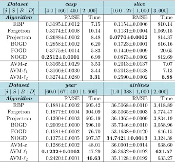
• Online regression: the regression task that follows the same setting of online classifi-cation, except the predictive performances are measured based on the regression error rate accumulated in the learning progress on the entire dataset.

(21)

Our main goal is to examine the scalability, classification and regression capabilities of AVMs by directly comparing with those of several recent state-of-the-art batch and online learning approaches using a number of datasets with a wide range of sizes. Our models are implemented in Python with Numpy package. The source code and experimental scripts are

published for reproducibility5. In what follows, we present the data statistics, experimental

setup, results and our observations.

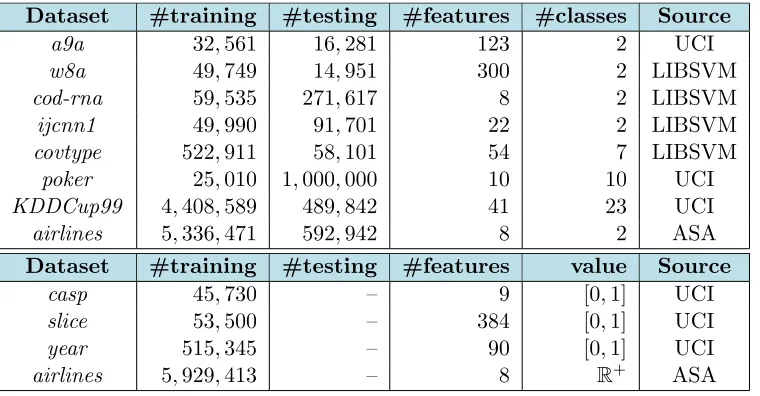
9.1 Data Statistics and Experimental Setup

We use 11 datasets whose statistics are summarized in Table 2. The datasets are selected in a diverse array of sizes in order to clearly expose the differences among scalable capabilities

of the models. Five of which (year, covtype, poker, KDDCup99, airlines) are large-scale

datasets with hundreds of thousands and millions of data points, whilst the rest are

ordinal-size databases. Except theairlines, all of the datasets can be downloaded from LIBSVM6

and UCI7 websites.

Dataset #training #testing #features #classes Source

a9a 32,561 16,281 123 2 UCI

w8a 49,749 14,951 300 2 LIBSVM

cod-rna 59,535 271,617 8 2 LIBSVM

ijcnn1 49,990 91,701 22 2 LIBSVM

covtype 522,911 58,101 54 7 LIBSVM

poker 25,010 1,000,000 10 10 UCI

KDDCup99 4,408,589 489,842 41 23 UCI

airlines 5,336,471 592,942 8 2 ASA

Dataset #training #testing #features value Source

casp 45,730 – 9 [0,1] UCI

slice 53,500 – 384 [0,1] UCI

year 515,345 – 90 [0,1] UCI

airlines 5,929,413 – 8 R+ ASA

Table 2: Data statistics. #training: number of training samples; #testing: number of testing samples.

The airlines dataset is provided by American Statistical Association (ASA8_{). The dataset}

contains information of all commercial flights in the US from October 1987 to April 2008. The aim is to predict whether a flight will be delayed or not and how long in minutes the flight will be delayed in terms of departure time. The departure delay time is provided in

the flight database. A flight is considereddelayed if its delay time is above 15 minutes, and

non-delayed otherwise. The average delay of a flight in 2008 was of 56.3 minutes. Following the procedure of (Hensman et al., 2013), we further process the data in two steps. First, we join the data with the information of individual planes basing on their tail numbers in order

5.https://github.com/tund/avm.

6._{https://www.csie.ntu.edu.tw/~cjlin/libsvmtools/datasets/}.

7.https://archive.ics.uci.edu/ml/datasets.html.

(22)

to obtain the manufacture year. This additional information is provided as a supplemental data source on ASA website. We then extract 8 features of many available fields: the age of the aircraft (computed based on the manufacture year), journey distance, airtime, scheduled departure time, scheduled arrival time, month, day of week and month. All features are

normalized into the range [0,1].

In batch classification experiments, we follow the original divisions of training and testing

sets in LIBSVM and UCI sites wherever available. For KDDCup99, covtype and airlines

datasets, we split the data into 90% for training and 10% for testing. In online classification and regression tasks, we either use the entire datasets or concatenate training and testing parts into one. The online learning algorithms are then trained in a single pass through the data. In both batch and online settings, for each dataset, the models perform 10 runs on different random permutations of the training data samples. Their prediction results and time costs are then reported by taking the average with the standard deviation of the results over these runs.

For comparison, we employ some baseline methods that will be described in the fol-lowing sections. Their C++ implementations with Matlab interfaces are published as a

part of LIBSVM, BudgetedSVM9 and LSOKL10 toolboxes. Throughout the experiments,

we utilize RBF kernel, i.e., Kx, x0 = exp

−γ

x−x

0

2

for all algorithms including

ours. We use hypersphere strategy to construct the δ-coverage (cf. Section 6.3), due to

its better performance than that of hyperrectangle approach during model evaluation. All experiments are conducted using a Windows machine with 3.46GHz Xeon processor and 96GB RAM.

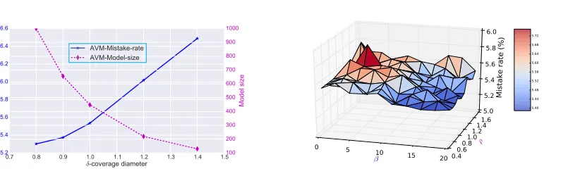
9.2 Model Evaluation on The Effect of Hyperparameters

In the first experiment, we investigate the effect of hyperparameters, i.e., δ-coverage

di-ameter, sampling parameters β and ρ (cf. Section 6.2.3) on the performance of AVMs.

Particularly, we conduct an initial analysis to quantitatively evaluate the sensitivity of these hyperparameters and their impact on the predictive accuracy and model size. This analysis provides a heuristic approach to find the best setting of hyperparameters. Here the AVM with Hinge loss is trained following the online classification scheme using two datasets

a9a and cod-rna.

To find the plausible range of coverage diameter, we use a heuristic approach as follows. First we compute the mean and standard deviation of pairwise Euclidean distances between any two data samples. Treating the mean as the radius, the coverage diameter is then varied around twice of this mean bounded by twice of the standard deviation. Fig. 2a and Fig. 3a report the average mistake rates and model sizes of AVMs with respect to (w.r.t) these

values for datasets a9a and cod-rna, respectively. Here we setβ = 0 andρ= 1.0. There is

a consistent pattern in both figures: the classification errors increase for largerδ whilst the

model sizes decrease. This represents the trade-off between model performance and model size via the model coverage. To balance the performance and model size, in these cases, we

can choose δ= 7.0 for a9a data andδ= 1.0 for cod-rna data.

9.http://www.dabi.temple.edu/budgetedsvm/index.html.

(23)

(a) The effect ofδ-coverage diameter on the mis-take rate and model size.

(b) The effect of β and ρ on the classification mistake rate. β= 0 means always approximating.

Figure 2: Performance evaluation of AVM with Hinge loss trained using a9a dataset with

different values of hyperparameters.

(a) The effect ofδ-coverage diameter on the mis-take rate and model size.

(b) The effect of β and ρ on the classification mistake rate. β= 0 means always approximating.

Figure 3: Performance evaluation of AVM with Hinge loss trained using cod-rna dataset

with different values of hyperparameters.

Fixing the coverage diameters, we vary β and ρ in 10 values monotonically increasing

from 0 to 10 and from 0.5 to 1.5, respectively, to evaluate the classification performance. The

smallerβand largerρindicate that the machine approximates the new incoming data more

frequently, resulting in less powerful prediction capability. This can be observed in Fig. 2b and Fig. 3b, which depict the average mistake rates in 3D as a function of these values for

dataseta9a andcod-rna. Hereβ = 0 means that the model always performs approximation

without respect to the value of ρ. From these visualizations, we found that the AVM with

always-on approximation mode still can achieve fairly comparable classification results.

Thus we setβ = 0 for all following experiments.

9.3 Batch Classification

We now examine the performances of AVMs in classification task following batch mode.

(24)

(delayed and non-delayed labels). We create two versions of our approach: AVM with Hinge loss (AVM-Hinge) and AVM with Logistic loss (AVM-Logit). It is noteworthy that the Hinge loss is not a smooth function with undefined gradient at the point that the classification

confidenceyf(x) = 1. Following the sub-gradient definition, in our experiment, we compute

the gradient given the condition that yf(x)<1, and set it to 0 otherwise.

Baselines. For discriminative performance comparison, we recruit the following state-of-the-art baselines to train kernel SVMs for classification in batch mode:

• LIBSVM: one of the most widely-used and state-of-the-art implementations for batch

kernel SVM solver (Chang and Lin, 2011). We use the one-vs-all approach as the default setting for the multiclass tasks;

• LLSVM: low-rank linearization SVM algorithm that approximates kernel SVM

opti-mization by a linear SVM using low-rank decomposition of the kernel matrix (Zhang et al., 2012);

• BSGD-M: budgeted stochastic gradient descent algorithm which extends the Pegasos

algorithm (Shalev-Shwartz et al., 2011) by introducing a merging strategy for support vector budget maintenance (Wang et al., 2012);

• BSGD-R: budgeted stochastic gradient descent algorithm which extends the Pegasos

algorithm (Shalev-Shwartz et al., 2011) by introducing a removal strategy for support vector budget maintenance (Wang et al., 2012);

• FOGD: Fourier online gradient descent algorithm that applies the random Fourier

features for approximating kernel functions (Lu et al., 2015);

• NOGD: Nystrom online gradient descent (NOGD) algorithm that applies the Nystrom

method to approximate large kernel matrices (Lu et al., 2015).

Hyperparameters setting. There are a number of different hyperparameters for all methods. Each method requires a different set of hyperparameters, e.g., the regularization

parameters (C in LIBSVM, λ in Pegasos and AVM), the learning rates (η in FOGD and

NOGD), the coverage diameter (δ in AVM) and the RBF kernel width (γ in all methods).

Thus, for a fair comparison, these hyperparameters are specified using cross-validation on training subset.

Particularly, we further partition the training set into 80% for learning and 20% for val-idation. For large-scale databases, we use only 1% of training set, so that the searching can finish within an acceptable time budget. The hyperparameters are varied in certain ranges and selected for the best performance on the validation set. The ranges are given as

fol-lows: C ∈

2−5,2−3, ...,215 ,λ∈ {2−4

/N,2−2/N, ...,216/N},γ ∈2−8,2−4,2−2,20,22,24,28 , η ∈ {16.0,8.0,4.0,2.0,0.2,0.02,0.002,0.0002} where N is the number of data points. The

coverage diameterδ of AVM is selected following the approach described in Section 9.2. For

the budget sizeB in NOGD and Pegasos algorithm, and the feature dimensionDin FOGD

(25)

Results. The classification results, training and testing time costs are reported in Table 3. Overall, the batch algorithms achieve the highest classification accuracies whilst those of online algorithms are lower but fairly competitive. The online learning models, however, are much sparser, resulting in a substantial speed-up, in which the training time costs and model sizes of AVMs are smallest with orders of magnitude lower than those of the standard batch methods. More specifically, the LIBSVM outperforms the other approaches in most of datasets, on which its training phase finishes within the time limit (i.e., two hours),

except for the ijcnn1 data wherein its testing score is less accurate but very close to that

of BSGD-M. The LLSVM achieves good results which are slightly lower than those of the state-of-the-art batch kernel algorithm. The method, however, does not support multiclass classification. These two batch algorithms – LIBSVM and LLSVM could not be trained

within the allowable amount of time on large-scale datasets (e.g., airlines), thus are not

scalable.

Furthermore, six online algorithms in general have significant advantages against the batch methods in computational efficiency, especially when running on large-scale datasets. Among these algorithms, the BSGD-M (Pegasos+merging) obtains the highest classification scores, but suffers from a high computational cost. This can be seen in almost all datasets, especially for the airlines dataset on which its learning exceeds the time limit. The slow

training of BSGD-M is caused by the merging step with computational complexityO B2

(B is the budget size). By contrast, the BSGD-R (Pegasos+removal) runs faster than the

merging approach, but suffers from very high inaccurate results due to its naive budget maintenance strategy, that simply discards the most redundant support vector which may contain important information.

In terms of predictive performance, our proposed methods outperform the recent ad-vanced online learning algorithms – FOGD and NOGD in most scenarios. The AVM-based models are able to achieve slightly less accurate but fairly comparable results compared with those of the state-of-the-art LIBSVM algorithm. In terms of sparsity and speed, the AVMs are the fastest ones in the training and testing phases in all cases thanks to their remarkable smaller model sizes. The difference between the training speed of our AVMs and that of two approaches varies across datasets. The gap is more significant for datasets with higher dimensional feature spaces. This is expected because the procedure to compute

random features for each data point of FOGD involves sin and cos operators which are

costly. These facts indicate that our proposed online kernel learning algorithms are both efficient and effective in solving large-scale kernel classification problems. Thus we believe that the AVM is the fast alternative to the existing SVM solvers for large-scale classification tasks.

(26)

Table 3: Classification performance of our AVMs and the baselines in batch mode. The

notation [δ|S |B|D], next to the dataset name, denotes the diameterδ, the model sizeS

of AVM-based models, the budget sizeB of budgeted algorithms, and the number of random

features D of FOGD, respectively. The accuracy is reported in percent (%), the training

time and testing time are in second. The best performance is inbold. It is noteworthy that

the LLSVM does not support multiclass classification and we terminate all runs exceeding the limit of two hours, therefore some results are unavailable.

Dataset [δ|S|B|D] a9a [7.0|135|1,000|4,000] w8a [13.0|131|1,000|4,000]

Algorithm Train Test Accuracy Train Test Accuracy

LIBSVM 84.57 22.23 84.92 50.96 2.95 99.06

LLSVM 50.73 8.73 83.00 92.19 10.41 98.64

BSGD-M 232.59 2.88 84.76±0.16 264.70 5.16 98.17±0.07 BSGD-R 90.48 2.72 80.26±3.38 253.30 4.98 97.10±0.04 FOGD 15.99 2.87 81.15±5.05 32.16 3.55 97.92±0.38 NOGD 82.40 0.60 82.33±2.18 374.87 0.65 98.06±0.18 AVM-Hinge 4.96 0.25 83.55±0.50 11.84 0.52 96.87±0.28 AVM-Logit 5.35 0.25 83.83±0.34 12.54 0.52 96.96±0.00

Dataset [δ|S|B|D] cod-rna [1.0|436|400|1,600] ijcnn1 [1.0|500|1,000|4,000]

LIBSVM 114.90 85.34 96.39 38.63 11.17 97.35

LLSVM 20.17 19.38 94.16 40.62 54.22 96.99

BSGD-M 90.62 5.66 95.67±0.21 93.05 6.13 97.69±0.11

BSGD-R 19.31 5.48 66.83±0.11 41.70 7.07 90.90±0.18 FOGD 7.62 11.95 92.65±4.20 7.31 10.10 90.64±0.07 NOGD 9.81 3.24 91.83±3.35 21.58 3.68 90.43±1.22 AVM-Hinge 6.52 2.69 94.38±1.16 6.47 2.71 91.14±0.71 AVM-Logit 7.03 2.86 93.10±2.11 6.86 2.67 91.19±0.95

Dataset [δ|S|B|D] covtype[3.0|59|400|1,600] poker [12.0|393|1,000|4,000]

LIBSVM – – – 40.03 932.58 57.91

LLSVM – – – – – –

BSGD-M 2,413.15 3.75 72.26±0.16 414.09 123.57 54.10±0.22 BSGD-R 418.68 3.02 61.09±1.69 35.76 102.84 52.14±1.05 FOGD 69.94 2.45 59.34±5.85 9.61 101.29 46.62±5.00 NOGD 679.50 0.76 68.20±2.96 118.54 36.84 54.65±0.27 AVM-Hinge 60.27 0.26 64.31±0.37 3.86 8.21 55.49±0.13 AVM-Logit 61.92 0.22 64.42±0.34 3.36 7.54 55.60±0.17

Dataset [δ|S|B|D] KDDCup99 [3.0|115|200|400] airlines [1.0|388|1,000|4,000]

LIBSVM 4,380.58 661.04 99.91 – – –

LLSVM – – – – – –

BSGD-M 2,680.58 21.25 99.73±0.00 – – –

BSGD-R 1,644.25 14.33 39.81±2.26 4,741.68 29.98 80.27±0.06 FOGD 706.20 22.73 99.75±0.11 1,085.73 861.52 80.37±0.21 NOGD 3,726.21 3.11 99.80±0.02 3,112.08 18.53 74.83±0.20 AVM-Hinge 554.42 2.75 99.82±0.05 586.90 6.55 80.72±0.00

(27)

9.4 Online Classification

The next experiment investigates the performance of the AVMs in online classification task where individual data point continuously come turn-by-turn in a stream. Here we also use eight datasets and two versions of our approach: AVM with Hinge loss (AVM-Hinge) and AVM with Logistic loss (AVM-Logit) which are used in batch classification setting (cf. Section 9.3).

Baselines. We recruit the two widely-used algorithms – Perceptron and OGD for regular online kernel classification without budget maintenance and 8 state-of-the-art budget online kernel learning methods as follows:

• Perceptron: the kernelized variant without budget of Perceptron algorithm (Freund

and Schapire, 1999);

• OGD: the kernelized variant without budget of online gradient descent (Kivinen et al.,

2004);

• RBP: a budgeted Perceptron algorithm using random support vector removal strategy

(Cavallanti et al., 2007);

• Forgetron: a kernel-based Perceptron maintaining a fixed budget by discarding oldest

support vectors (Dekel et al., 2005);

• Projectron: a Projectron algorithm using the projection strategy (Orabona et al.,

2009);

• Projectron++: the aggressive version of Projectron algorithm (Orabona et al., 2009);

• BPAS: a budgeted variant of Passive-Aggressive algorithm with simple SV removal

strategy (Wang and Vucetic, 2010);

• BOGD: a budgeted variant of online gradient descent algorithm using simple SV

removal strategy (Zhao et al., 2012);

• FOGD and NOGD: described in Section 9.3.

Hyperparameters setting. For each method learning on each dataset, we follow the same hyperparameter setting which is optimized in the batch classification task. For time efficiency, we only include the fast algorithms FOGD, NOGD and AVMs for the experiments on large-scale datasets. The other methods would exceed the time limit when running on such data.

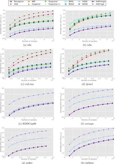
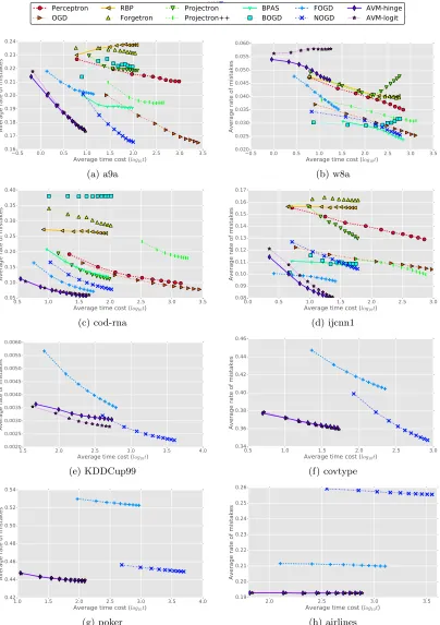
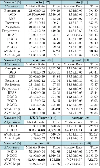
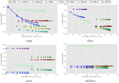
Results. Fig. 4 and Fig. 5 shows the relative performance convergence w.r.t classification error and computation cost of the AVMs in comparison with those of the baselines. Com-bining these two figures, we compare the average mistake rate and running time in Fig. 6. Table 4 reports the final average results in detailed numbers after the methods see all data

samples. It is worthy to note that for the four biggest datasets (KDDCup99,covtype,poker,

(28)

First of all, as can be seen from Fig. 4, there are three groups of algorithms that have different learning progresses in terms of classification mistake rate. The first group includes the BOGD, Projectron and Forgetron that have the error rates fluctuating at the beginning, but then being stable till the end. In the meantime, the rates of the models in the second group, including Perceptron, OGD, RBP, Projectron++ and BPAS, quickly saturate at a plateau after these methods see a few portions, i.e., one-tenth to two-tenth, of the data. By contrast, the last group includes the recent online learning approaches – FOGD, NOGD, and our proposed ones – AVM-Hinge, AVM-Logit, that regularly perform better as more data

points come. Exceptionally, for the dataset w8a, the classification errors of the methods in

the first group keep increasing after seeing four-tenth of the data, whilst those of the last group are unexpectedly worse.

Second, Fig. 6 plots average mistake rate against computational cost, which shows sim-ilar patterns as in the our first observation. In addition, it can be seen from Fig. 5 that all algorithms have normal learning pace in which the execution time is accumulated over the learning procedure. Only the Projectron++ is slow at the beginning but then performs faster after receiving more data.

According to final results summarized in Table 4, the budgeted online approaches show efficacies with substantially faster computation than the ones without budgets. This is more obvious for larger datasets wherein the execution time costs of our proposed models are several orders of magnitude lower than those of regular online algorithms. This is because the coverage scheme of AVMs impressively boost their model sparsities, e.g., using

δ= 3 resulting in 115 core points for datasetKDDCup99 consisting of 4,408,589 instances,

and usingδ = 1 resulting in 388 core points for datasetairlines containing 5,336,471 data

samples.

For classification capability, the non-budgeted methods only surpass the budgeted ones

for the smallest dataset, that is, the OGD obtains the best performance fora9a data. This

again demonstrates the importance of exploring budget online kernel learning algorithms. Between the two non-budgeted algorithms, the OGD achieves considerably better error rates than the Perceptron. The method, however, must perform much more expensive updates, resulting in a significantly larger number of support vectors and significantly higher computational time costs. This represents the trade-off between classification accuracy and computational complexity of the OGD.

Furthermore, comparing the performance of different existing budgeted online kernel learning algorithms, the AVM-Hinge and AVM-Logit outperform others in both discrimi-native performance and computation efficiency for almost all datasets. In particular, the

AVM-based methods achieve the best mistake rates – 5.61±0.17, 8.01±0.18, 43.85±0.09,

19.28±0.00 for the cod-rna, ijcnn1, poker and airlines data, that are, respectively, 27.5%,

17.5%, 2.4%, 8.8% lower than the error rates of the second best models – two recent

ap-proaches FOGD and NOGD. On the other hand, the computation costs of the AVMs are

significantly lower with large margins of hundreds of percents for large-scale databases

(29)

Approximation Vector Machines

0 1 2 3 4 5

Number of samples ×104

0.16 0.17 0.18 0.19 0.20 0.21 0.22

Average rate of mistakes

Perceptron