Iranian Chemical Society
Anal. Bioanal. Chem. Res., Vol. 6, No. 1, 111-124, June 2019.
Characterization of Binary Edible Oil Blends Using Color Histograms and Pattern
Recognition Techniques
Shiva Ahmadi
a,*, Ahmad Mani-Varnosfaderani
b,* and Buick Habibi
aa
Department of Chemistry, Faculty of Science, Azarbaijan Shahid Madani University, Tabriz, 53714-161, Iran.
bDepartment of Chemistry, Tarbiat Modares University, Tehran, Iran
(Received 22 April 2018, Accepted 26 August 2018)
Nutritionalvalue and quality features of oils are the most important factors that should be considered in food industry. There is no pure
edible oil with the appropriate oxidative stability and nutritional properties. Therefore, vegetable oils are blended to improve their
applications and to enhance their nutritional quality. Characterization of edible oils is important for quality control and identification of oil adulteration. In this work, we propose a simple, rapid, inexpensive and non-destructive approach for characterization of different types of
vegetable oil blends according to the corresponding color histograms. Regression models were applied on four datasets of binary edible oil blends including palm olein-rapeseed, palm olein-sunflower, soybean-sunflower, and soybean-rapeseed. In all of the aforementioned data sets, despite the high performances of the support vector regression (SVR), and Levenberg-Marquardt artificial neural network (LMANN)
regression models in terms of coefficient of determination, Bayesian regularized artificial neural networks (BRANN) provided better results up to 97% for HSI color histograms in both the training and test sets. In order to reduce the numbers of independent variables for
modelling, principal component analysis (PCA) algorithm was used. Finally, the results of image analysis were compared with those obtained by processing of FT-IR spectra of mixtures of edible oils. The results revealed that image analysis of mixtures of edible oils yield comparable results to those obtained by processing of FT-IR spectra for characterization of edible oils. Our results suggest that the
proposed method is promising for characterization of different binary blends of edible oils.
Keywords: Multivariate calibration, Edible oil analysis, Image histograms, Artificial neural networks, Bayesian regularization
INTRODUCTION
Edible oils are used for cooking and frying in food product preparation. There are three factors that are commonly considered while choosing an appropriate oil: quality, stability and nutritional features. Because of the specific chemical and physical properties, most of the vegetable oils have restricted technological applications in their original forms [1]. To increase the application of vegetable oils, they are upgraded using different approaches; hydrogenation, interesterification, fractionation
*Corresponding authors. E-mail: ahmadishiva_ch@yahoo. com; [email protected]
sunflower, and soybean have wide applications to achieve different aims such as increasing nutritional value, reducing the cost and meet demands in the food industry in many countries [7]. There are many reports that palm, rapeseed, sunflower, and soybean blending are used in the edible oil industry [8-11].
Different methodologies such as chemometrics, pattern recognition, and image analysis techniques have been planned to determine the physical/chemical properties of food. Nowadays, digital image processing is becoming more important because of its ability to perform fast and non-invasive low-cost analysis on products and materials [12]. Digital image processing has successfully been used for classification of honey [13], Coffee [14], bacteria [15], tea [16], vegetable oil [17], bio-diesels [18], propolis [19] and motor oil [20]. To the best of our knowledge, the present work is the first report to address the characterization problem of blended edible oils based on image processing techniques. We applied the proposed image analysis technique on the binary mixture that are most commonly used in blended edible oils in the food industry in many countries: palm olein-rapeseed, palm olein-sunflower, soybean-sunflower, and soybean- rapeseed. To this end, we extract a set of features of images based on three color spaces including: red green blue (RGB), hue saturation intensity (HSI), and grayscale. The RGB color space is based on the mechanism of human visual system, where radiations of different colors are provided by combination of different levels of light radiation at red, green and blue. The HSI system is more representative of the way humans perceive colors, and sometimes it is also more convenient for image processing. The HSI color model represents every color with three components: hue, saturation, and intensity. The hue component describes the color itself (e.g., red or yellow), saturation refers to how much the color is polluted with white color, and intensity indicates brightness [17,21]. The use of this color space in the field of color image analysis has already given quite satisfactory results. The basic problem addressed in this paper is the regression problem. Regression analysis can be defined as the process of developing a mathematical model that can be used to predict one variable by using another variable (s). Regression therefore aims to fit a line or curve through the data in order to describe the relationship between some
variables [22]. In this work Bayesian regularized artificial neural networks (BRANN), Levenberg-Marquardt artificial neural network (LMANN), and support vector regression (SVR) techniques are employed for characterization and identification of blended edible oils. We use regression as an approach to model the relationship between blended components in edible blended oils. For training the regression models we use the separated groups, including binary mixtures of x 0% - y 100%, x 25% - y 75%, x 50% - y 50%, x 75% - y 25% and x 100% - y 0% of edible oils where x and y are two components of binary edible oil blends. These combination models are applied on four data sets of binary edible oil blends including palm olein-rapeseed, palm olein-sunflower, soybean-sunflower, and soybean-rapeseed.
Support vector machine (SVM) is a supervised machine learning algorithm that can be used for both classification and regression. This method characterizes using kernels and subset of training points in the decision function (called support vectors), so, it is also memory efficient. The goal of SVM method is minimizing the generalization error bound in order to achieve a generalized performance. The idea of SVR is based on the computation of a non-linear regression using what is called the kernel trick, implicitly mapping their inputs into high-dimensional feature spaces [23]. The research has shown that neural networks are valuable in fitting models to data containing interactions. The goal of training the network is to change the weights between the layers in direction to minimize the output errors [24]. In this study we use Levenberg-Marquardt and Bayesian regularized algorithms for training the networks in the regression processes.
Additionally, principal component analysis (PCA) algorithm is used for reducing the number of independent variables for regression analysis. The PCA method defines some limited number of latent variables used as the input vectors for development of the appropriate BRANN, LRANN and SVR models. Monte-Carlo cross validation (MCCV) strategy is used for parameter optimization of the neural network models including numbers of neurons in hidden layers and numbers of independent variables. MCCV technique is also used for optimization of kernel parameters in SVR models.
summary of the materials and methods in Section 2, the experimental results and discussion are presented in Section 3, and the conclusion in Section 4.
MATERIALS AND METHODS
Samples
Edible oil contains a variety of components which all play a part in its refinement. In commercial processes, edible oil is colorless, odorless, and flavorless. The main steps of an edible oil refining process include [25]: 1) Degumming: The phosphatides in crude oil are reduced, 2) Neutralizing: The free acids of oil are neutralized by using alkali, 3) Deodorizing: Odor and taste are removed under high temperature and sparge steam condition, and 4) Winterizing: Un-pleasant turbidity components like waxes at low temperature are eliminated. After refining process, in this work, a total of 75 samples of the most common used blended edible oils including palm, rapeseed, sunflower, and soybean were analyzed. For image acquisition, 15.0 ml of each sample was used to fill a Petri plate 80 mm × 15 mm in order to promote uniformity, and to maintain the overall visual characteristics of the sample surface.
Apparatus
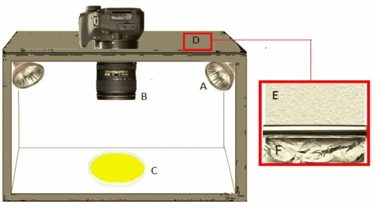
The apparatus used for image capturing was built using a Styrofoam box with the size of 70 cm × 40 cm × 40 cm externally covered with aluminum foil to avoid stray light interferences, ensuring the uniformity of the captured image. A 25 MP Nikon camera (D5300, DLSR) with a 23.5 × 15.6 mm sensor size was allocated in the center of the box and above the sample holder, vertically. The distance between the camera and the sample holder was 35 cm. Two LED lamps of 3W were placed in two sides of the wall at an angle of 45 degree. The main architecture of the image acquisition system is illustrated in Fig. 1.
Acquisition of Image Histograms
Color histograms describe the statistical distribution of the pixels as a function of color space channels. In this work, each color component of the Grayscale, RGB, and HSV systems is composed of 256 tones [26-30] and the signal magnitude in these channels were used as analytical information. In order to extract features from samples,
different color channels (R, G, B, H, S, I) and their combinations were selected.
In this work, a total of 375 images (5 images for each sample of binary edible oil) were obtained. Then, a region of interest (ROI) with 1000 × 1000 pixels was selected at the center of each image. Since color histograms describe statistical distribution of colors in pixels, the selection of ROI provides enough information to obtain a suitable regression model. In the matrix of the data set, the data in rows correspond to samples, and columns represent the constituted variables corresponding to the color levels obtained for each color component. Figure 2 illustrates the procedure of mean histogram acquisition in the grayscale, red, green, blue, hue, saturation, and intensity channels.
Principal Component Analysis
The principal component analysis (PCA) algorithm is a statistical procedure that uses an orthogonal transformation to convert an N-dimensional data into an M-dimensional one (M < N). This transformation is defined in such a way that the first PC takes as high variance as possible, and each succeeding component in turn finds the highest variance under the constraint that it must be orthogonal to the preceding components. The use of the PCA algorithm is greatly accepted for visualization of large databases. This method is widely used for visualization and reduction of the data set dimension [31-33].
Regression Methods
Two different types of regression models have been used in this work for regression of binary blended edible oils. The first method is support vector regression (SVR), and the next group used is ANN algorithms which are one of the most popular data mining approaches and are well known for their ability to model nonlinear characteristics in data sets. The research has shown that a neural network with a sufficient number of parameters can model any continuous nonlinear function accurately. Some authors also showed that neural networks are valuable in fitting models to data containing interactions [34]. Following sections are devoted to description of SVR and ANN algorithms used in this study for blended edible oil analysis.
Fig. 1. Apparatus built for image capturing of of binary edible oil blends samples; (A) LED lamp, (B) Camera, (C) Sample
holder, (D) Surface of the box, (E) Styrofoam layer, and (F) Aluminum foil layer.
the input space of the sample and has a corresponding target value yi Rn for i = 1,…, n, where n corresponds to the size of the training data [23,35]. The idea of the regression problem is to determine a function that can approximate future values accurately. The generic SVR estimating function takes the form:
f(x) = (w . (x)) + b (1)
where w Rn, b Rn and denotes a non-linear transformation from Rn to high dimensional space. The main goal is to find the value of w and b such that values of x can be determined by minimizing the regression risk:
1 2 1 1 2 1 ) ) (
(f x y w
C
Rreg
i i (2)
where C is a constant determining penalties to estimate errors. The vector w can be written in terms of data points as:
1 ( ) ( )
1 i
i i i x
w
(3)By substituting Eq. (3) into Eq. (1), the generic equation can be rewritten as:
f x i xi x b
i i
( )( ( ). ( )) )( 1
1 (4)
k x x b
i i
i i
11( ) ( , ) (4')
In Eq. (4), the dot product can be replaced with function k(xi,x), known as the kernel function. Kernel functions enable dot product to be performed in high-dimensional feature space using low dimensional space data input without knowing the transformation . Some common kernels are [36,37]:
the radial basis function (RBF),
2
exp ) ,
(xi x x xi
k (5)
the polynomial function,
di
i x x x
x
k( ) ( )1 (6)
and the linear function,
k(xi,x)x.y (7)
In Eq. (2), is a cost function. The -insensitive loss function is widely used as a cost function [35,38]. The
-insensitive loss function is in the form of:
f x y for f x y
otherwise
y x
f () , ( ()
0 ) ) (
( (8)
Artificial neural networks. Artificial neural networks
are nonlinear statistical data modeling tools through them the complex relationships between inputs and outputs are modeled, or patterns are found. Since artificial neural networks are not restricted to linear correlations, they can be used for nonlinear phenomena or curved manifold. In analytical applications, back propagation neural networks (BNNs) are the most common methods for training the neural networks. The back propagation network receives a set of inputs, that are multiplied by each node, and then a nonlinear transfer function is applied [39,40]. In a supervised training, both the inputs and the outputs are provided. The network then processes the inputs and compares its resulting outputs against the desired outputs. Errors are then propagated back through the system; making the system adjust the weights controlling the network. There are many algorithms for training multilayer perceptrons such as gradient descent, variable learning rate gradient descent, conjugate gradient descent, Newton algorithms, and faster quasi-Newton algorithms such as levenberg-marquardt. In this study, we used Bayesian regularization and Levenberg-Marquardt algorithms for training the networks. The detailed discussion about training algorithms for ANN can be found elsewhere [24,41].
Regularization in ANN models. The aim of
regularization in ANN models is adjusting the performance function, which is usually considered to be the mean sum of squares of training samples errors (mse) and is defined by the following equation.
N i i e N mse 1 2 ) (1 (9)
the performance function by adding the mean square of weights (msw) calculated by the following equation:
msereg = αmse + βmsw (10)
where α and β are performance ratios, and msw is the mean square of weights calculated by Eq. (11).
1 1 2 1 i j w Nmse (11)
Using this performance function makes the networks’ weights and biases smaller, leading to the smoother network
response that is less likely over-fitted. The problem with regularization is the difficulty in determining the optimum value for the performance ratio parameter. One approach to determine the optimum value of performance ratio is Bayesian framework of David MacKay [42].
The BRANN, LMANN and SVR algorithms were
implemented using the standard codes of MATLAB software (2016a, version 9.0). The calculations were carried out on a desktop computer with ‘Windows 7 Pro’ as the operating system, Intel(R) Core(TM) core i7 CPU and 8GB of RAM memory.
RESULTS AND DISCUSSION
Exploratory Data Analysis
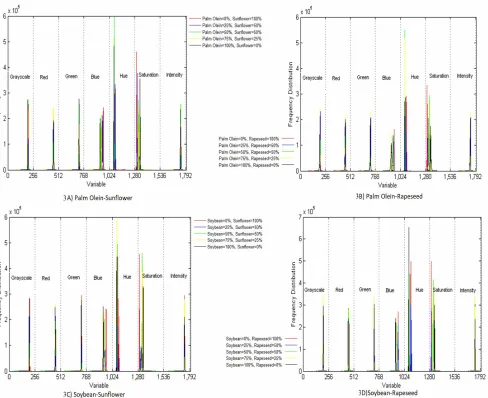
The mean histograms of binary edible oil blends including palm olein-rapeseed, palm olein-sunflower, soybean -sunflower and soybean- rapeseed are illustrated in
Figs. 3A-3D, respectively. As can be seen, the mean histograms exhibited notable separations respect to their compositions in the blue, saturation and hue channels. Moreover, samples are relatively separated into five major groups of x 0% - y 100%, x 25% - y 75%, x 50% - y 50%, x
75% - y 25% and x 100% - y 0% where x and y are two components of binary edible oil blends.
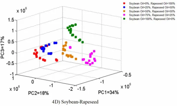
After collection of the data, a 375 × 1729 data matrix has been built and used for further analysis. PCA algorithm was used for analysis of the collected data matrix. Figures 4A-4D illustrate the 3D-scatter plots made by the first three
PC scores using RGB+HSI+Grayscale channels for palm
olein-rapeseed, palm olein-sunflower, soybean-sunflower and soybean-rapeseed blends, respectively. These score plots for PC1-PC3 are especially useful, since these three components summarize more variations in the data than any other combination of PCs, and give the information about the patterns hidden in the dataset. As can be seen in Fig. 4,
samples are separated in five major groups using the data acquired by combination of RGB+HIS+Grayscale channels. The data in Fig. 4 reveals that samples are reasonably separated according to their edible oil compositions. The separated groups in Fig. 4 include binary mixtures of x 0% -
y 100%, x 25% - y 75%, x 50% - y 50%, x 75% - y 25% and x 100% - y 0% of edible oils where x and y are two components of binary edible oil blends. It can be seen that the combination of RGB+HIS+Grayscale color spaces provide high discriminatory power with low overlaps for separating different percentages of the blends of the edible
oils.
After exploring the discriminatory power of different color spaces (and their combinations) using PCA algorithm, three different pattern recognition techniques were used to develop regression models for precise characterization of the blends of edible oils. In this respect, SVR, BRANN and
LMANN regression models were implemented using the individual channels and their combinations. PCA was used to reduce the number of independent variables for model development. Monte-Carlo cross validation strategy was also used to find the best numbers of PCs for development of supervised models.
Regression Modeling
1 ) (
1
2 , mod ,
n x x RMSE
n
i obsi eli (12)
where xobs is observed values, and xmodel is the modeled
value for sample number ( i ).
n
i
n
i eli el
obs i obs n
i obsi obs obsi el
x x x
x
x x x x R
1 1
2 mod , mod 2
,
2
1 , , mod
2
) (
. ) (
) (
. )
( (13)
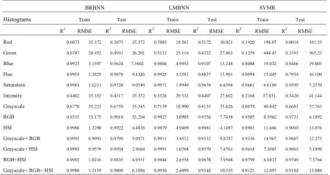
The results of the BRANN, LMANN and SVR techniques for modeling the fraction of edible oils in binary mixtures in training and test sets are given in Tables 1-4 for palm olein-rapeseed, palm olein-sunflower, soybean-sunflower and soybean-rapeseed mixtures, respectively. As can be seen in these tables, combinations of RGB, Grayscale and HIS channels provide necessary information for correct determination of the fraction of edible oils in binary mixtures. Moreover, inspection of Tables 1-4 reveals that BRANN algorithm is superior over optimized LMANN and
Fig. 3. Mean histograms of the binary edible oil blends in the grayscale, red, green, blue, hue, saturation and
intensity channels for A) palm olein-sunflower, B) palm olein-rapeseed, C) Soybean-Sunflower and D)
Fig. 4. Scatter plots of the first three PCs using RGB+HIS+Grayscale data for 4A) palm olein-sunflower, 4B)
Fig. 4. Continued.
Table 1. The Fitness Values (RMSE) and Coefficient of Determination (R2) Obtained Using BRANN, LMANN and SVR Algorithms for Modeling the Composition of Different Mixtures of Palm Olein and Rapeseed Oils
BRANN LMANN SVR
Histograms Train Test Train Test Train Test
R2 RMSE R2 RMSE R2 RMSE R2 RMSE R2 RMSE R2 RMSE Red 0.6754 35.364 0.1546 35.366 0.6186 22.753 0.0257 40.988 0.0524 108.23 0.0707 122.04
Green 0.5025 35.212 0.4937 35.253 0.6589 20.716 0.4856 32.283 0.1368 284.75 0.4314 480.68
Blue 0.9994 0.8532 0.9445 11.843 0.9852 4.3252 0.8305 19.851 0.9721 6.3420 0.9144 11.630
Hue 0.9875 4.0311 0.9850 6.2649 0.9793 5.3188 0.8157 24.504 0.0537 44.603 0.0519 51.259
Saturation 0.9992 1.0521 0.9428 22.988 0.9963 2.1845 0.9453 13.151 0.9757 5.7470 0.9700 7.7357
Intensity 0.4176 35.356 0.1437 35.356 0.6904 19.732 0.1463 40.532 0.1618 514.82 0.5097 519.16
Grayscale 0.7736 17.199 0.7277 18.752 0.8255 15.558 0.4798 31.189 0.0002 229.19 0.2027 456.64
RGB 0.9951 2.5510 0.9642 8.7202 0.9839 4.6092 0.8966 20.026 0.9533 8.9909 0.8378 16.267
HSI 0.9988 1.2404 0.9767 5.6409 0.9530 7.8503 0.9505 9.1977 0.9786 8.6141 0.9833 8.7464
Grayscale+ RGB 0.9908 3.4748 0.8698 12.833 0.9555 7.6924 0.8156 15.918 0.8761 19.084 0.6371 24.860
Grayscale+ HSI 0.9981 1.5844 0.9789 7.5037 0.9457 8.6588 0.8737 17.336 0.9814 6.6186 0.9773 6.9692
RGB+HSI 0.9998 0.5736 0.9746 8.0014 0.9955 2.4513 0.8845 12.525 0.9682 6.7161 0.9683 7.7695
Table 2. The Fitness Values (RMSE) and Coefficient of Determination (R2) Obtained Using BRANN, LMANN and SVR Algorithms for Modeling the Composition of Different Mixtures of Palm Olein and Sunflower Oils
BRANN LMANN SVR
Histograms Train Test Train Test Train Test
R2 RMSE R2 RMSE R2 RMSE R2 RMSE R2 RMSE R2 RMSE Red 0.3964 35.358 0.0633 35.369 0.3265 30.139 0.0647 62.831 0.0068 74.291 0.0086 56.507
Green 0.7391 35.496 0.5966 35.495 0.7105 20.747 0.3791 35.761 0.5187 116.96 0.5876 111.12
Blue 0.9995 0.3229 0.9807 6.7989 0.9860 4.2600 0.9214 14.135 0.9440 14.701 0.9110 14.648
Hue 0.9866 4.1511 0.9015 13.869 0.9535 7.6312 0.9418 19.340 0.8211 18.903 0.9111 17.976
Saturation 0.9998 0.4637 0.9579 15.226 0.9984 1.4373 0.9326 10.637 0.9849 4.7384 0.9859 4.8847
Intensity 0.6642 35.383 0.7383 35.382 0.7786 17.055 0.3174 33.251 0.4037 580.14 0.7621 601.13
Grayscale 0.8322 14.584 0.6115 27.663 0.7794 16.712 0.5150 28.265 0.1601 50.934 0.0286 60.102
RGB 0.9989 1.1928 0.9080 11.419 0.9757 5.5885 0.9772 6.7838 0.9698 7.0896 0.9904 7.6321
HSI 0.9995 0.8229 0.9726 22.591 0.9584 7.2646 0.9013 15.703 0.9780 5.4354 0.9797 5.5158
Grayscale+ RGB 0.9982 1.5264 0.9621 8.5795 0.9911 3.3460 0.9177 10.566 0.8618 18.439 0.9567 18.633
Grayscale+ HSI 0.9999 0.3692 0.9566 8.5394 0.9934 3.0661 0.9756 6.2335 0.8878 15.709 0.8765 17.745
RGB+HSI 0.9997 0.6421 0.9206 18.196 0.9943 2.6944 0.9212 11.334 0.9720 10.360 0.9909 8.9926
Grayscale+ RGB+ HSI 0.9998 0.4546 0.9538 10.864 0.9915 3.3868 0.9661 8.2349 0.9524 9.4968 0.9645 9.7917
Table 3. The Fitness Values (RMSE) and Coefficient of Determination (R2) Obtained Using BRANN, LMANN and SVR
Algorithms for Modeling the Composition of Different Mixtures of Soybean and Sunflower Oils
BRBNN LMBNN SVMR
Histograms Train Test Train Test Train Test
R2 RMSE R2 RMSE R2 RMSE R2 RMSE R2 RMSE R2 RMSE Red 0.6073 35.372 0.3875 35.372 0.7085 19.561 0.5172 30.021 0.1920 194.07 0.0014 181.55
Green 0.6747 20.452 0.4931 26.201 0.5121 25.116 0.4332 27.863 0.1259 444.47 0.3391 565.23
Blue 0.9923 3.1597 0.9624 7.5602 0.9804 4.9953 0.9107 13.248 0.8088 19.032 0.8466 19.003
Hue 0.9955 2.3825 0.9878 9.4326 0.9925 3.1581 0.8637 13.901 0.8094 15.445 0.7934 16.100
Saturation 0.9981 1.6211 0.9728 9.0549 0.9971 1.9949 0.9674 6.6394 0.9661 6.6189 0.9595 7.2570
Intensity 0.4402 35.352 0.4317 35.352 0.3526 29.532 0.4407 27.602 0.2168 37.831 0.3428 41.144
Grayscale 0.6770 35.221 0.6759 35.245 0.7159 18.990 0.4133 35.626 0.6074 40.842 0.6681 37.763
RGB 0.9315 35.175 0.9018 35.204 0.9927 3.0905 0.9556 7.7438 0.9505 8.3962 0.9731 6.1892
HSI 0.9986 1.3290 0.9922 4.4838 0.9879 4.0409 0.9881 4.1497 0.8981 11.666 0.9003 13.076
Grayscale+ RGB 0.9991 0.9991 0.9799 5.0971 0.9911 3.4512 0.9332 9.6787 0.9336 14.967 0.9807 12.275
Grayscale+ HSI 0.9993 0.9579 0.9934 2.9684 0.9991 1.0708 0.9570 7.6761 0.9618 7.3081 0.9803 5.1898
RGB+HSI 0.9992 1.0216 0.9835 4.9551 0.9944 2.6558 0.9678 7.9504 0.9799 6.8817 0.9749 7.3764
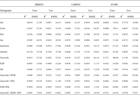
Table 4. The Fitness Values (RMSE) and Coefficient of Determination (R2) Obtained Using BRANN, LMANN and SVR Algorithms for Modeling the Composition of Different Mixtures of Soybean and Rapeseed Oils
BRBNN LMBNN SVMR
Histograms Train Test Train Test Train Test
R2 RMSE R2 RMSE R2 RMSE R2 RMSE R2 RMSE R2 RMSE Red 0.8619 12.583 0.8087 16.673 0.8026 16.351 0.4654 26.682 0.8005 19.012 0.7714 19.606
Green 0.3032 35.383 0.0567 35.383 0.5496 27.421 0.0336 60.207 0.0000 789.51 0.0697 815.65
Blue 0.9766 5.4269 0.9606 8.0522 0.9456 8.4783 0.7308 20.559 0.8547 15.781 0.8822 13.960
Hue 0.9995 0.8191 0.9419 10.933 0.9972 1.9099 0.9804 9.6855 0.9073 12.342 0.9172 12.504
Saturation 0.9998 0.5448 0.9932 4.7944 0.9998 0.5184 0.9431 10.375 0.9679 6.7122 0.9695 6.4728
Intensity 0.3724 35.336 0.1209 35.349 0.6686 21.676 0.1518 59.051 0.0616 34.293 0.0030 35.562
Grayscale 0.4415 35.365 0.3482 35.365 0.6018 23.827 0.2664 44.152 0.1371 480.60 0.1196 530.84
RGB 0.9907 3.4345 0.9888 14.426 0.9856 4.3510 0.9565 11.137 0.9163 10.458 0.9385 8.9510
HSI 0.9996 0.7737 0.9844 5.4877 0.9919 3.5519 0.9579 9.1670 0.9798 7.1467 0.9754 7.5057
Grayscale+ RGB 0.9908 3.4034 0.9553 7.9141 0.9656 7.8005 0.8229 15.063 0.4649 29.827 0.5965 28.566
Grayscale+ HSI 0.9994 0.8759 0.9918 11.189 0.9703 6.5857 0.9014 17.030 0.9868 4.2301 0.9906 3.5293
RGB+HSI 0.9994 0.8569 0.9894 9.8339 0.9840 4.5741 0.9629 11.542 0.9661 8.9894 0.9593 9.6038
Grayscale+ RGB+ HSI 0.9985 1.3832 0.9937 8.9635 0.9903 3.5271 0.9278 10.569 0.9791 6.8745 0.9796 7.0127
Table 5. The Fitness Values (RMSE) and Coefficient of Determination (R2) Obtained Using BRANN Algorithm for Modeling the Composition of Four Binary Mixtures of Edible Oils Using FT-IR
Data in the Ranges of 400-4000 cm-1
Oil Mixture Training Test
R2 RMSE R2 RMSE
Palm Olein-Rapeseeda 0.983 2.742 0.968 4.184
Palm Olein-Sunflower 0.979 2.450 0.984 3.944
Soybean-Sunflower 0.990 1.792 0.973 2.859
Soybean-Rapeseed 0.983 2.050 0.966 4.160
a
The numbers of optimized PCs for characterization of Palm Olein-Rapeseed, Palm Olein-Sunflower, Soybean-Sunflower, Soybean-Rapeseed mixtures were 8, 7, 12 and 8 respectively. Monte Carlo cross
SVR algorithms for modeling the data. This is mainly due to the automatic regularization in BRANN networks handled by Bayes probability theorem. The regularized BRANN models are general and can be used for prediction of unseen objects in test sets, and therefore return better results than those obtained by SVR and LMANN algorithms.
Comparison of Image Histograms with FT-IR Data
To further investigate the performance of the developed method, the trained BRANN models (as the best models) were compared with those trained with the FT-IR spectra of binary edible oils. In this respect, a total of 375 FT-IR spectra in the ranges of 400-4000 cm-1 were obtained formixtures of binary edible oil blends using a Thermo Scientific Nicolet IR100 (Madison, WI, USA) FT-IR spectroscopy. 50 µl of edible oils was blended with potassium bromide powder (KBr) and compressed as tablets, and then FT-IR spectra were obtained with Nicolet IR 100 Thermo. All spectra were corrected against a background air spectrum and gathered as transmittance values at each data point. The FT-IR spectra for different blends of binary edible oils including soybean-rapeseed, soybean-sunflower, palm-rapeseed, and palm-sunflower are illustrated in Figs. 5a-d, respectively. PCA algorithm was used for reducing the number of independent variables for modeling, and MCCV approach was used for selecting the
Fig. 5. The FT-IR spectra for different blends of binary edible oils including (a) Soybean-Rapeseed, (b) Soybean-
best sets of PCs to be used as input for BRANN algorithm. Also, the numbers of neurons in the hidden layer were optimized using MCCV approach. The results of BRANN regression algorithm for modeling the fractions of oils in blends of palm olein-rapeseed, palm olein-sunflower, soybean-sunflower, and soybean-rapeseed mixtures are given in Table 5. As can be seen in this table, the results of BRANN models trained by FT-IR spectra are comparable to those obtained using BRANN models trained with images of the mixtures of edible oils. This finding suggests that the proposed image analysis approach in this work can be used as a simple alternative tool to FT-IR spectroscopy for modeling the composition of different mixtures of binary edible oils.
CONCLUSIONS
Most vegetable oils have limited technological applications in their original forms because of their specific chemical and physical properties. To enhance their commercial applications, vegetable oils are often modified using blending. This paper proposed a simple and non-expensive methodology based on digital images and pattern recognition techniques for the characterization of the binary blends of the most common used edible oils. Different color histograms of grayscale, RGB and HSI color channels and also their combination were used as inputs for modeling using BRANN, LMANN and SVR regression methods. These regression models were applied on 4 data sets of binary edible oil blends including palm olein-rapeseed, palm olein-sunflower, sunflower and soybean-rapeseed. In all of the aforementioned data sets, despite the high performance of SVR and LMANN regression models in terms of coefficient of determination, BRANN provided better results up to 97% for HSI color histograms in both the training and test sets. The results in this work revealed that the proposed BRANN models trained by digital image histograms are comparable to those trained by FT-IR for characterization of binary mixtures of edible oils. The results in this contribution suggest that the proposed method can be used as a simple quality control approach in oil analysis laboratories. This method does not need complex pretreatment procedures and huge amounts of solvents usually consumed during oil characterization procedures in
oil industry.
ACKNOWLEDGEMENTS
The authors are grateful to the Research Office of Azarbaijan Shahid Madani University, Tabriz, Iran and Tarbiat Modares University for financial supports.
Compliance with Ethical Standards
Funding. The authors would like to thank the research
council of Tarbiat Modares University and Azarbaijan Shahid Madani University for financial support of this project.
Conflict of interest. Shiva Ahmadi declares that she has
no conflict of interest. Ahmad Mani-Varnosfaderani declares that he has no conflict of interest. Buick Habibi declares that he has no conflict of interest.
Ethical approval. This article does not contain any
studies with human participants or animals performed by any of the authors.
Informed Consent. Not applicable.
REFERENCES
[1] F. Gunstone, Vegetable Oils in Food Technology: Composition, Properties and Uses, Wiley-Blackwell, 2011.
[2] F. Hashempour-Baltork, M. Torbati, S. Azadmard-Damirchi, G.P. Savage, Trends Food Sci. Tech. 57 (2016) 52.
[3] N.A. Idris, N.L.H.M. Dian, Asia Pac. J. Clin. Nutr. 14 (2005) 396.
[4] S.M. Downs, V. Gupta, S. Ghosh-Jerath, K. Lock, A.M. Thow, A. Singh, BMC Public Health 13 (2013) 1139.
[5] R.V. Rios, M.D.F. Pessanha, P.F. de Almeida, C.L. Viana, S.C. da S. Lannes, Food Sci. Technol. Campinas 34 (2014) 3.
[6] T.-T. Xu, J. Li, Y.-W. Fan, T.-W. Zheng, Z.-Y. Deng, Int. J. Food Prop. 18 (2015) 1478.
[7] R.S. Farag, M.A. El-Agaimy, B.S.A. El Hakeem, Food Nutr. Sci. 1 (2010) 24.
[9] E. De Marco, M. Savarese, C. Parisini, I. Battimo, S. Falco, R. Sacchi, Eur. J. Lipid Sci. Tech. 109 (2007) 237.
[10] H. Sakurai, J. Pokorný, Eur. J. Lipid. Sci. Technol. 105 (2003) 769
[11] M. Naghshineh, A.A. Ariffin, H.M. Ghazali, H. Mirhosseini, A.S. Mohammad, A. Kuntom, J. Food Lipids 16 (2009) 554.
[12] R.C. Gonzalez, R.E. Woods, Digital Image Processing,) 3rd Edition, Prentice Hall, 2008. [13] M.A. Domínguez, P.H.G.D. Diniz, M.S. DiNezio,
M.C.U. Araújo, M.E. Centurión, Microchem. J. 112 (2014) 104.
[14] U.T.C.P. Souto, M.F. Barbosa, H.V. Dantas, A.S. Pontes, W.S. Lyra, P.H.G.D. Diniz, M.C.U. Araújo, E.C. Silva, Food Anal. Methods 8 (2015) 1515. [15] V.E. Almeida, G.B. Costa, D.D.S. Fernandes,
P.H.G.D. Diniz, D. Brandão, A.C.D. Medeiros, G. Véras, Anal. Bioanal. Chem. 406 (2014) 5989. [16] P.H.G.D. Diniz, H.V. Dantas, K.D.T. Melo, M.F.
Barbosa, D.P. Harding, E.C.L. Nascimento, M.F. Pistonesi, B.S.F. Band, M.C.U. Araújo, Anal. Methods 4 (2012) 2648.
[17] K.D.T.M. Milanez, M.J.C. Pontes, Microchem. J. 113 (2014) 10.
[18] G.B. Costa, D.D.S. Fernandes, V.E. Almeida, T.S.P. Araújo, J.P. Melo, P.H.G.D. Diniz, G. Véras, Talanta 139 (2015) 50.
[19] G.D. Pierini, D.D.S. Fernandes, P.H.G.D. Diniz, M.C.U. De Araújo, M.S. Di Nezio, M.E. Centurión, Microchem. J. 128 (2016) 62.
[20] S. Ahmadi, A. Mani-Varnosfaderani, B. Habibi, J. AOAC Int. 101 (2018) xx.
[21] K. Plataniotis, A.N. Venetsanopoulos, Color Image Processing and Applications. Springer Science and Business Media, 2013.
[22] N.R. Draper, H. Smith, Applied Regression Analysis, John Wiley and Sons, 2014
[23] A.J. Smola, B. Scholkopf, Stat. Comput. 14 (2004) 199.
[24] Y. Anzai, Pattern Recognition and Machine Learning, Elsevier, 2012.
[25] A.J.C. Andersen, Refining of Oils and Fats for Edible Purposes, Elsevier, 2016.
[26] A. Choodum, P. Kanatharana, W. Wongniramaikul, N.N. Daeid, Talanta 115 (2013) 143.
[27] C. Duchesne, J. Liu, J.F. Mac Gregor, Chemometr. Intell. Lab. 117 (2012) 116.
[28] S.W. Lyra, L.F. Almeida, F.A.S. Cunha, P.H.G.D. Diniz, V.L. Martins, M.C.U. Araújo, Anal. Methods 6 (2014) 1044.
[29] C.L.M. Morais, K.M.G. Lima, Talanta 126 (2014) 145.
[30] P.M. Santos, E.R. Pereira-Filho, Anal. Methods 5 (2013) 3669.
[31] R.V. Deursen, L.C. Blum, J. Reymond, J. Chem. Inf. Model 50 (2010) 1924.
[32] D. Hiristozov, T.I. Oprea, J. Gasteiger, J. Chem. Inf. Model 47 (2007) 2044.
[33] M. Jalali-Heravi, A. Mani-Varnosfaderani, Mol. Inform. 31 (2012) 63.
[34] L.P.J. Veelenturf, Analysis and Applications of Artificial Neural Networks. Prentice-Hall, 1995. [35] Vladimir N. Vapnik, The Nature of Statistical
Learning Theory, Springer-Verlag Berlin, Heidelberg ©1995.
[36] B. Scholkopf, A.J. Smola, Learning with Kernels: Support Vector Machines, Regularization, Optimization, and Beyond. MIT Press, 2001.
[37] J. Li, IEEE Trans. Instrum. Meas. 59 (2010) 2094. [38] R.M. Balabin, E.I. Lomakina, Analyst 136 (2011)
1703.
[39] F.R. Burden, D.A. Winkler, J. Med. Chem. 42 (199) 3183.
[40] M. Jalali-Heravi, A. Mani-Varnosfaderani, Mol. Inform. 28 (2009) 946.