Vol. 4, No. 3, Year 2012 Article ID IJIM-00283, 20 pages Research Article
Numerical Solution of Sawada-Kotera equation by
using Iterative Methods
Sh. Sadigh Behzadi∗
Department of Mathematics, Islamic Azad University, Qazvin Branch, Qazvin, Iran.
——————————————————————————————————
Abstract
In this paper, the Sawada-Kotera equation is solved by using the Adomian’s decomposition method, modified Adomian’s decomposition method, variational iteration method, mod-ified variational iteration method, homotopy perturbation method, modmod-ified homotopy perturbation method and homotopy analysis method. The approximate solution of this equation is calculated in the form of series which its components are computed by applying a recursive relation. The existence and uniqueness of the solution and the convergence of the proposed methods are proved. A numerical example is studied to demonstrate the accuracy of the presented methods.
Keywords : Sawada-Kotera equation; Adomian decomposition method; Modified Adomian de-composition method; Variational iteration method (VIM), Modified variational iteration method; Homotopy perturbation method; Modified homotopy perturbation method; Homotopy analysis method.
——————————————————————————————————
1
Introduction
In recent years, some works have been done in order to find the numerical solution of the Sawada-Kotera equation. For example [1, 2, 3, 4, 5, 6, 7, 8, 9, 10]. In this work, we develope the ADM, MADM, VIM, MVIM, HPM, MHPM and HAM to solve this equation as follows:
ut+ 45u2ux−15uxuxx−15uuxxx+uxxxxx= 0, (1.1) with the initial condition:
u(x,0) =f(x), (1.2) ∗Corresponding author. Email address: shadan [email protected] .
where subscripts denote the derivatives of the corresponding variable, which is widely used in many branches of physics such as conformal field theory, two-dimensional quan-tum gravitation canonical field theory, the conservation flow of the Liouville equation in nonlinear science [43] , and so on. The paper is organized as follows. In section 2, the mentioned iterative methods are introduced for solving Eq.(1.1). In section 3 we prove the existence , uniqueness of the solution and convergence of the proposed methods. Finally, the numerical example and computational complexity of the proposed methods are shown in section 4. In order to obtain an approximate solution of Eq.(1.1), let us integrate one time Eq.(1.1) with respect tot using the initial condition we obtain,
u(x, t) = (1.3)
f(x)−45
∫ t
0
F1(u(x, τ)dτ+15
∫ t
0
F2(u(x, τ))dτ+15
∫ t
0
F3(u(x, τ))dτ−
∫ t
0
F4(u(x, τ))dτ,
where,
F1(u(x, t)) =u2(x, t)D(u(x, t)), F2(u(x, t)) =D(u(x, t))D2(u(x, t)), F3(u(x, t)) =u(x, t)D3(u(x, t)), F4(u(x, t)) =D5(u(x, t)),
Di(u(x, t)) = ∂iu∂x(x,ti ), i= 1,2,3,5.
In Eq.(1.3), we assume f(x) is bounded for all x in J = [0, T](T ∈ R). The terms
F1(u(x, t)),F2(u(x, t)),F3(u(x, t)), andF4(u(x, t)) are Lipschitz continuous with|F1(u)− F1(u∗)|≤L1|u−u∗ |,|F2(u)−F2(u∗)|≤L2|u−u∗ |,|F3(u)−F3(u∗)|≤L3 |u−u∗ |
and |F4(u)−F4(u∗)|≤L4 |u−u∗|.
2
The iterative methods
2.1 Description of the MADM and ADM
The Adomian decomposition method is applied to the following general nonlinear equation
Lu+Ru+N u=g1, (2.4)
whereu(x, t) is the unknown function,Lis the highest order derivative operator which is assumed to be easily invertible,R is a linear differential operator of order less thanL, N u
represents the nonlinear terms, and g1 is the source term. Applying the inverse operator L−1 to both sides of Eq.(2.4), and using the given conditions we obtain
u(x, t) =f1(x)−L−1(Ru)−L−1(N u), (2.5)
where the functionf1(x) represents the terms arising from integrating the source termg1.
The nonlinear operator N u=G1(u) is decomposed as
G1(u) =
∞
∑
n=0
An, (2.6)
where An, n≥0 are the Adomian polynomials determined formally as follows :
An= 1
n![
dn dλn[N(
∞
∑
i=0
The first Adomian polynomials (introduced in [11, 12, 13]) are:
A0 =G1(u0), A1 =u1G′1(u0), A2 =u2G′1(u0) +
1 2!u
2
1G′′1(u0), (2.8) A3 =u3G′1(u0) +u1u2G′′1(u0) +
1 3!u
3
1G′′′1(u0), ...
2.1.1 Adomian decomposition method
The standard decomposition technique represents the solution ofu(x, t) in Eq.(2.4) as the following series,
u(x, t) =
∞
∑
i=0
ui(x, t), (2.9)
where, the componentsu0, u1, . . . which can be determined recursively u0 =f(x),
u1 =−45
∫ t
0
A0(x, t)dt+ 15
∫ t
0
B0(x, t) dt+ 15
∫ t
0
L0(x, t) dt−
∫ t
0
S0(x, t) dt,
.. .
un+1 =−45
∫ t
0
An(x, t) dt+ 15
∫ t
0
Bn(x, t)dt+ 15
∫ t
0
Ln(x, t) dt−
∫ t
0
Sn(x, t) dt n≥0. (2.10) Substituting Eq.(2.8) into Eq.(2.10) leads to the determination of the components ofu.
2.1.2 The modified Adomian decomposition method
The modified decomposition method was introduced by Wazwaz [14]. The modified forms was established on the assumption that the function f(x) can be divided into two parts, namely f1(x) and f2(x). Under this assumption we set
f(x, t) =f1(x) +f2(x). (2.11)
Accordingly, a slight variation was proposed only on the components u0 and u1. The
suggestion was that only the part f1 be assigned to the zeroth component u0, whereas
the remaining part f2 be combined with the other terms given in Eq.(2.11) to defineu1.
Consequently, the modified recursive relation
u0 =f1(x),
u1 =f2(x)−L−1(Ru0)−L−1(A0), (2.12)
.. .
was developed. To obtain the approximation solution of Eq.(1.1), according to the MADM, we can write the iterative formula Eq.(2.12) as follows:
u0 =f1(x), u1 =f2(x)−45
∫t
0A0(x, t)dt+ 15
∫t
0B0(x, t) dt+ 15
∫t
0 L0(x, t) dt−
∫t
0S0(x, t))dt,
.. .
un+1=−45
∫t
0An(x, t) dt+ 15
∫t
0Bn(x, t) dt+ 15
∫t
0Ln(x, t) dt−
∫t
0Sn(x, t)) dt, n≥1.
(2.13) The operatorsFi(u(x, t)) (i= 1,2,3,4) are usually represented by the infinite series of the Adomian polynomials as follows:
F1(u) =
∞
∑
i=0 Ai,
F2(u) =
∞
∑
i=0 Bi,
F3(u) =
∞
∑
i=0 Li,
F4(u) =
∞
∑
i=0 Si,
where Ai , Bi, Li and Si are the Adomian polynomials. Also, we can use the following formula for the Adomian polynomials [15]:
An =F1(sn)−
∑n−1
i=0 Ai, Bn=F2(sn)−
∑n−1
i=0 Bi,
Ln=F3(sn)−
∑n−1
i=0 Li,
Sn=F4(sn)−
∑∞
i=0Si.
(2.14)
Where sn=
∑n
i=0ui(x, t) is the partial sum. 2.2 Description of the VIM and MVIM
In the VIM [16, 17, 18, 19, 20, 35, 41, 42], it has been considered the following nonlinear differential equation:
Lu+N u=g1, (2.15)
where L is a linear operator, N is a nonlinear operator and g1 is a known analytical
function. In this case, the functions un may be determined recursively by
un+1(x, t) =un(x, t)+
∫ t
0
λ(x, τ){L(un(x, τ))+N(un(x, τ))−g1(x, τ)}dτ, n≥0, (2.16)
will be readily obtained upon using the obtained Lagrange multiplier and by using any selective functionu0. The zeroth approximationu0 may be selected any function that just
satisfies at least the initial and boundary conditions. With λ determined, then several approximation un(x, t), n≥0 follow immediately. Consequently, the exact solution may be obtained by using
u(x, t) = lim
n→∞un(x, t). (2.17) The VIM has been shown to solve effectively, easily and accurately a large class of nonlin-ear problems with approximations converge rapidly to accurate solutions. To obtain the approximation solution of Eq.(1.1), according to the VIM, we can write iteration formula Eq.(2.16) as follows:
un+1(x, t) =un(x, t) +Lt−1(λ[un(x, t)−f(x) + 45
∫t
0F1(un(x, t))dt
−15∫0tF2(un(x, t))dt−15
∫t
0 F3(un(x, t))dt+
∫t
0F4(un(x, t))dt]), n≥0.
(2.18)
Where,
L−t1(.) =
∫ t
0
(.)dτ.
To find the optimalλ, we proceed as
δun+1(x, t) =δun(x, t) +δLt−1(λ[un(x, t)−f(x) + 45
∫t
0F1(un(x, t))dt
−15∫0tF2(un(x, t)) dt−15
∫t
0F3(un(x, t))dt+
∫t
0F4(un(x, t))dt]).
(2.19)
From Eq.(2.19), the stationary conditions can be obtained as follows: λ′ = 0 and 1+λ= 0. Therefore, the Lagrange multipliers can be identified as λ = −1 and by substituting in Eq.(2.18), the following iteration formula is obtained.
u0(x, t) =f(x),
un+1(x, t) =un(x, t)−Lt−1(un(x, t)−f(x) + 45
∫t
0F1(un(x, t))dt
−15∫0tF2(un(x, t))dt−15
∫t
0 F3(un(x, t))dt+
∫t
0F4(un(x, t))dt), n≥0.
(2.20)
To obtain the approximation solution of Eq.(1.1), based on the MVIM [21, 22, 23], we can write the following iteration formula:
u0(x, t) =f(x),
un+1(x, t) =un(x, t)−L−t1(45
∫t
0 F1(un(x, t)−un−1(x, t))dt
−15∫0tF2(un(x, t)−un−1(x, t))dt−15
∫t
0F3(un(x, t)−un−1(x, t)) dt+
∫t
0F4(un(x, t)−un−1(x, t))dt), n≥0.
(2.21)
Relations Eq.(2.20) and Eq.(2.21) will enable us to determine the components un(x, t) recursively for n≥0.
2.3 Description of the HAM
Consider
N[u] = 0,
parameter, H1(x, t)̸= 0 an auxiliary function, andLan auxiliary linear operator with the
propertyL[s(x, t)] = 0 whens(x, t) = 0. Then usingq ∈[0,1] as an embedding parameter, we construct a homotopy as follows:
(1−q)L[ϕ(x, t;q)−u0(x, t)]−qhH1(x, t)N[ϕ(x, t;q)] = ˆH[ϕ(x, t;q);u0(x, t), H1(x, t), h, q].
(2.22) It should be emphasized that we have great freedom to choose the initial guessu0(x, t), the
auxiliary linear operatorL, the non-zero auxiliary parameterh, and the auxiliary function
H1(x, t). Enforcing the homotopy Eq.(2.22) to be zero, i.e.,
ˆ
H1[ϕ(x, t;q);u0(x, t), H1(x, t), h, q] = 0, (2.23)
we have the so-called zero-order deformation equation
(1−q)L[ϕ(x, t;q)−u0(x, t)] =qhH1(x, t)N[ϕ(x, t;q)]. (2.24)
Whenq = 0, the zero-order deformation Eq.(2.24) becomes
ϕ(x; 0) =u0(x, t), (2.25)
and whenq= 1, sinceh̸= 0 and H1(x, t)̸= 0, the zero-order deformation Eq.(2.24) is
equivalent to
ϕ(x, t; 1) =u(x, t). (2.26) Thus, according to Eq.(2.25) and Eq.(2.26), as the embedding parameter q increases from 0 to 1,ϕ(x, t;q) varies continuously from the initial approximationu0(x, t) to the
ex-act solutionu(x, t). Such a kind of continuous variation is called deformation in homotopy [23, 24, 25, 26, 40].
Due to Taylor’s theorem, ϕ(x, t;q) can be expanded in a power series of q as follows
ϕ(x, t;q) =u0(x, t) +
∞
∑
m=1
um(x, t)qm, (2.27)
where,
um(x, t) = 1
m!
∂mϕ(x, t;q)
∂qm |q=0.
Let the initial guessu0(x, t), the auxiliary linear parameter L, the nonzero auxiliary
parameter h and the auxiliary function H1(x, t) be properly chosen so that the power
series Eq.(2.27) of ϕ(x, t;q) converges at q = 1, then, we have under these assumptions the solution series
u(x, t) =ϕ(x, t; 1) =u0(x, t) +
∞
∑
m=1
um(x, t). (2.28)
From Eq.(2.27), we can write Eq.(2.24) as follows
(1−q)L[ϕ(x, t, q)−u0(x, t)] = (1−q)L[
∑∞
m=1um(x, t) qm] =q h H1(x, t)N[ϕ(x, t, q)]⇒ L[∑∞m=1um(x, t) qm]−q L[∑∞m=1um(x, t)qm] =q h H1(x, t)N[ϕ(x, t, q)]
By differentiating Eq.(2.29)m times with respect toq, we obtain
{L[∑∞m=1um(x, t) qm]−q L[∑∞m=1um(x, t)qm]}(m)={q h H1(x, t)N[ϕ(x, t, q)]}(m) = m!L[um(x, t)−um−1(x, t)] =h H1(x, t) m ∂
m−1N[ϕ(x,t;q)] ∂qm−1 |q=0 . Therefore,
L[um(x, t)−χmum−1(x, t)] =hH1(x, t)ℜm(um−1(x, t)), (2.30)
where,
ℜm(um−1(x, t)) =
1 (m−1)!
∂m−1N[ϕ(x, t;q)]
∂qm−1 |q=0, (2.31)
and
χm=
{
0, m≤1 1, m >1
Note that the high-order deformation Eq.(2.30) is governing the linear operatorL, and the term ℜm(um−1(x, t)) can be expressed simply by Eq.(2.31) for any nonlinear operator N.
To obtain the approximation solution of Eq.(1.1), according to HAM, let
N[u(x, t)] =
u(x, t)−f(x) + 45∫0tF1(u(x, t)) dt−15
∫t
0F2(u(x, t))dt−15
∫t
0F3(u(x, t))dt
+∫0tF4(u(x, t))dt,
so,
ℜm(um−1(x, t)) = um−1(x, t)−f(x) + 45
∫t
0 F1(um−1(x, t))dt−15
∫t
0 F2(um−1(x, t))dt
−15∫0tF3(um−1(x, t))dt+
∫t
0 F4(um−1(x, t))dt.
(2.32)
Substituting Eq.(2.32) into Eq.(2.30)
L[um(x, t)−χmum−1(x, t)] =hH1(x, t)[um−1(x, t)−f(x) + 45
∫t
0F1(um−1(x, t))dt
−15∫0tF2(um−1(x, t))dt−15
∫t
0F3(um−1(x, t))dt
+∫0tF4(um−1(x, t))dt.+ (1−χm)f(x)(x)].
(2.33) We take an initial guessu0(x, t) =f(x), an auxiliary linear operatorLu=u, a nonzero
auxiliary parameter h=−1, and auxiliary functionH1(x, t) = 1. This is substituted into
Eq.(2.33) to give the recurrence relation
u0(x, t) =f(x),
un+1(x, t) =−45
∫t
0F1(un(x, t))dt+ 15
∫t
0F2(un(x, t))dt+ 15
∫t
0F3(un(x, t))dt
−∫t
0 F4(un(x, t))dt, n≥0.
Therefore, the solutionu(x, t) becomes
u(x, t) =∑∞n=0un(x, t) =f(x) +∑∞n=1( −45∫0tF1(un(x, t)) dt (2.35)
+15
∫ t
0
F2(un(x, t))dt+ 15
∫ t
0
F3(un(x, t)) dt−
∫ t
0
F4(un(x, t))dt). Which is the method of successive approximations. If
|un(x, t)|<1,
then the series solution Eq.(2.35) convergence uniformly.
2.4 Description of the HPM and MHPM
To explain HPM [27, 28, 34, 36, 37, 38, 39], we consider the following general nonlinear differential equation:
Lu+N u=f(u), (2.36) with initial conditions
u(x,0) =f(x).
According to HPM, we construct a homotopy which satisfies the following relation
H(u, p) =Lu−Lv0+p Lv0+p [N u−f(u)] = 0, (2.37)
where p ∈ [0,1] is an embedding parameter and v0 is an arbitrary initial approximation
satisfying the given initial conditions.
In HPM, the solution of Eq.(2.37) is expressed as
u(x, t) =u0(x, t) +p u1(x, t) +p2 u2(x, t) +... (2.38)
Hence the approximate solution of Eq.(2.36) can be expressed as a series of the power of
p, i.e.
u= lim
p→1u=u0+u1+u2+...
where,
u0(x, t) =f(x),
.. .
um(x, t) =∑mk=0−1−45∫0tF1(um−k−1(x, t))dt+ 15
∫t
0 F2(um−k−1(x, t))dt+
15∫0tF3(um−k−1(x, t))dt−
∫t
0F4(um−k−1(x, t)) dt, m≥1.
(2.39)
To explain MHPM [30, 31, 32], we consider Eq.(1.1) as
L(u) =u(x, t)−f(x) + 45∫0tF1(um−k−1(x, t))dt−15
∫t
0F2(um−k−1(x, t))dt
−15∫0tF3(um−k−1(x, t))dt+
∫t
0F4(um−k−1(x, t)) dt.
WhereF1(u(x, t)) =g1(x)h1(t),F2(u(x, t)) =g2(x)h2(t), F3(u(x, t)) =g3(x)h3(t) and F4(u(x, t)) =g4(x)h4(t). We can define homotopyH(u, p, m) by
where, m is an unknown real number and
f(u(x, t)) =u(x, t)−z(x, t).
Typically we may choose a convex homotopy by
H(u, p, m) = (1−p)f(u) +p L(u) +p (1−p)[m(g1(x) +g2(x) +g3(x))] = 0, 0≤p≤1.
(2.40) Wherem is called the accelerating parameters, and for m= 0 we define H(u, p,0) =
H(u, p),which is the standard HPM.
The convex homotopy Eq.(2.40) continuously trace an implicity defined curve from a starting pointH(u(x, t)−f(u),0, m) to a solution functionH(u(x, t),1, m).The embedding parameterpmonotonically increase from 0 to 1 as trivial problemf(u) = 0 is continuously deformed to original problemL(u) = 0.
The MHPM uses the homotopy parameterpas an expanding parameter to obtain
v=
∞
∑
n=0
pnun, (2.41)
whenp→1, Eq.(2.37) corresponds to the original one and Eq.(2.41) becomes the approx-imate solution of Eq.(1.1), i.e.,
u= lim p→1v=
∞
∑
m=0 um.
Where,
u0(x, t) =f(x), u1(x, t) =
−45∫0tF1(u0(x, t)) dt+ 15
∫t
0F2(u0(x, t)) dt+ 15
∫t
0F3(u0(x, t)) dt−
∫t
0F4(u0(x, t)) dt
−m(g1(x) +g2(x) +g3(x) +g4(x)), u2(x, t) =
−45∫0tF1(u1(x, t)) dt+ 15
∫t
0F2(u1(x, t)) dt+ 15
∫t
0F3(u1(x, t)) dt−
∫t
0F4(u1(x, t)) dt
+m(g1(x) +g2(x) +g3(x) +g4(x)),
.. .
um(x, t) =
∑m−1
k=0 −45
∫t
0F1(um−k−1(x, t))dt+ 15
∫t
0 F2(um−k−1(x, t))dt+
15∫0tF3(um−k−1(x, t))dt−
∫t
0F4(um−k−1(x, t)) dt, m≥3.
(2.42)
3
Existence and convergency of iterative methods
We set,
α1 :=T(45L1+ 15L2+ 15L3+L4),
Theorem 3.1. Let 0< α1<1, then Sawada-Kotera Eq.(1.1), has a unique solution.
Proof. Letu and u∗ be two different solutions of Eq.(1.3) then
|u−u∗ |=| −45∫0t[F1(u(x, t))−F1(u∗(x, t))] dt+ 15
∫t
0[F2(u(x, t))−F2(u∗(x, t))]dt
+15∫0t[F3(u(x, t))−F3(u∗(x, t))] dt−
∫t
0 F4(u(x, t))dt|
≤45∫0t|F1(u(x, t))−F1(u∗(x, t))| dt+ 15
∫t
0 |F2(u(x, t))−F2(u∗(x, t))| dt+
15∫0t|F3(u(x, t))−F3(u∗(x, t))| dt+
∫t
0 |F4(u(x, t))| dt
≤T(L1+L2+L3+L4) |u−u∗ |=α1 |u−u∗|.
From which we get (1−α1)|u−u∗ |≤0. Since 0< α1 <1, then|u−u∗ |= 0. Implies u=u∗ and completes the proof. 2
Theorem 3.2. The series solution u(x, t) =∑∞i=0ui(x, t) of Eq.(1.1) using MADM con-vergence when
0< α1 <1,|u1(x, t)|<∞.
Proof. Denote as (C[J],∥.∥) the Banach space of all continuous functions on J with the norm ∥ f(t) ∥= max | f(t) |, for all t in J. Define the sequence of partial sums sn, let sn and sm be arbitrary partial sums with n≥m. We are going to prove that sn is a Cauchy sequence in this Banach space:
∥sn−sm∥=
max∀t∈J |sn−sm |=max∀t∈J |
∑n
i=m+1ui(x, t)|= max∀t∈J | −45
∫t
0(
∑n−1
i=mAi) dt+ 15
∫t
0(
∑n−1
i=mBi) dt+ 15∫0t(∑ni=−m1Li)dt−
∫t
0(
∑n−1
i=mSi)dt|. From [15], we have
∑n−1
i=mAi =F1(sn−1)−F1(sm−1),
∑n−1
i=mBi =F2(sn−1)−F2(sm−1),
∑n−1
i=mLi =F3(sn−1)−F3(sm−1),
∑n−1
i=mSi =F4(sn−1)−F4(sm−1).
So,
∥sn−sm ∥=
max∀t∈J | −45
∫t
0[F1(sn−1)−F1(sm−1)]dt+ 15
∫t
0[F2(sn−1)−F2(sm−1)]dt+ 15
∫t
0[F3(sn−1)−F3(sm−1)]dt−
∫t
0[F4(u(x, t))−F4(u(x, t))]dt|≤
45∫0t|F1(sn−1)−F1(sm−1)| dt+ 15
∫t
0 |F2(sn−1)−F2(sm−1)| dt
+15∫0t|F3(sn−1)−F3(sm−1)| dt+
∫t
0 |F4(sn−1)−F4(sm−1) dt≤α1∥sn−sm∥.
Letn=m+ 1, then
∥sn−sm∥≤α1 ∥sm−sm−1 ∥≤α21 ∥sm−1−sm−2∥≤...≤αm1 ∥s1−s0 ∥.
∥sn−sm∥≤∥sm+1−sm∥+∥sm+2−sm+1∥+...+∥sn−sn−1∥
≤[αm1 +αm1+1+...+α1n−m−1]∥s1−s0∥
≤αm1 [1 +α1+α21+...+α1n−m−1]∥s1−s0 ∥≤αm1 [
1−αn1−m
1−α1 ]∥u1(x, t)∥. Since 0< α1 <1, we have (1−αn1−m)<1, then
∥sn−sm ∥≤
αm1
1−α1
max∀t∈J |u1(x, t)|. (3.43)
But | u1(x, t) |< ∞ , so, as m → ∞, then ∥ sn−sm ∥→ 0. We conclude that sn is a Cauchy sequence in C[J], therefore the series is convergence and the proof is complete.
2
Theorem 3.3. The maximum absolute truncation error of the series solution u(x, t) =
∑∞
i=0ui(x, t)to Eq.(1.1) by using MADM is estimated to be
max|u(x, t)− m
∑
i=0
ui(x, t)|≤
kαm1
1−α1
. (3.44)
Proof. From inequality Eq.(3.44), when n→ ∞, then sn→u and
max|u1(x, t)|
≤T(45max∀t∈J |F1(u0(x, t))|+
15max∀t∈J |F2(u0(x, t))|+15max∀t∈J |F3(u0(x, t))|+max∀t∈J |F4(u0(x, t))|).
Therefore,
∥u(x, t)−sm∥≤ αm1
1−α1T(45max∀t∈J |F1(u0(x, t))|+
15max∀t∈J |F2(u0(x, t))|+15max∀t∈J |F3(u0(x, t))|+max∀t∈J |F4(u0(x, t))|).
Finally the maximum absolute truncation error in the intervalJis obtained by Eq.(3.45). Theorem 3.4. The solution un(x, t) obtained from the relation Eq.(2.20) using VIM converges to the exact solution of the Eq.(1.1) when 0< α1 <1 and 0< β1 <1.
Proof.
un+1(x, t) =un(x, t)−Lt−1([un(x, t)−f(x) + 45
∫t
0F1(un(x, t))dt−15
∫t
0F2(un(x, t))dt
−15∫0tF3(un(x, t))) dt+
∫t
0F4(un(x, t))dt])
(3.45)
u(x, t) =u(x, t)−L−t1([u(x, t)−f(x) + 45∫0tF1(u(x, t))dt−15
∫t
0 F2(u(x, t))dt
−15∫0tF3(u(x, t))) dt+
∫t
0F4(u(x, t))dt])
un+1(x, t)−u(x, t) =un(x, t)−u(x, t)−L−t1(un(x, t)−u(x, t) +45∫0t[F1(un(x, t))−F1(u(x, t))] dt−15
∫t
0[F2(un(x, t))−F2(u(x, t))]dt−
15∫0t[F3(un(x, t))−F3(u(x, t))] dt+
∫t
0[F4(un(x, t))−F4(un(x, t)) dt),
if we set, en+1(x, t) = un+1(x, t)−un(x, t), en(x, t) = un(x, t)−u(x, t),| en(x, t∗) |=
maxt | en(x, t) | then since en is a decreasing function with respect to t from the mean value theorem we can write,
en+1(x, t) =en(x, t) +Lt−1(−en(x, t)−45
∫t
0[F1(un(x, t))−F1(u(x, t))]dt
+15∫0t[F2(un(x, t))−F2(u(x, t))] dt+ 15
∫t
0[F3(un(x, t))−F3(u(x, t))]dt−
∫t
0[F4(un(x, t))−F4(u(x, t))] dt)
≤en(x, t) +L−t1[−en(x, t) +L−t1 |en(x, t)|(T(45L1+ 15L2+ 15L3+L4)]
≤en(x, t)−T en(x, η) +T(45L1+ 15L2+ 15L3+L4)L−t1Lt−1 |en(x, t)|
≤(1−T(1−α1)|en(x, t∗)|,
where 0≤η≤t. Hence,en+1(x, t)≤β1 |en(x, t∗)|. Therefore,
∥en+1∥=max∀t∈J |en+1|≤β1 max∀t∈J |en|≤β1∥en∥.
Since 0 < β1 < 1, then ∥en∥ → 0. So, the series converges and the proof is complete.
2
Theorem 3.5. The solution un(x, t) obtained from the Eq.(2.22) using MVIM for the Eq.(1.1) converges when 0< α1 <1 , 0< γ1 <1.
Proof. The Proof is similar to the previous theorem.
Theorem 3.6. The maximum absolute truncation error of the series solution u(x, t) =
∑∞
i=0ui(x, t)to Eq.(1.1) by using VIM is estimated to be
∥en∥ ≤
β1nk′
1−β1
, k′ =max|u1(x, t)|.
Proof.
un+1−un= (un+1−u) + (u−un) =en−en+1
→en=en+1−(un+1−un)
∥en∥=∥en+1−(un+1−un)∥ ≤ ∥en+1∥+∥un+1−un∥ ≤β1∥en∥+∥un+1−un∥
→ ∥en∥ ≤ ∥un1+1−β1−un∥ ≤ β
n
1k ′
1−β1. 2
Theorem 3.7. If the series solution Eq.(2.34) of Eq.(1.1) using HAM convergent then it converges to the exact solution of the Eq.(1.1).
Proof. We assume:
u(x, t) =∑∞m=0um(x, t),
b
F1(u(x, t)) =
∑∞
m=0F1(um(x, t)),
b
F2(u(x, t)) =
∑∞
m=0F2(um(x, t)),
b
F3(u(x, t)) =
∑∞
m=0F3(um(x, t)),
b
F4(u(x, t)) =
∑∞
Where,
lim
m→∞um(x, t) = 0. We can write,
n
∑
m=1
[um(x, t)−χmum−1(x, t)] =u1+ (u2−u1) +...+ (un−un−1) =un(x, t). (3.47)
Hence, from Eq.(3.47),
lim
n→∞un(x, t) = 0. (3.48) So, using Eq.(3.48) and the definition of the linear operatorL, we have
∞
∑
m=1
L[um(x, t)−χmum−1(x, t)] =L[
∞
∑
m=1
[um(x, t)−χmum−1(x, t)]] = 0.
therefore from , we can obtain that,
∞
∑
m=1
L[um(x, t)−χmum−1(x, t)] =hH1(x, t)
∞
∑
m=1
ℜm−1(um−1(x, t)) = 0.
Sinceh̸= 0 and H1(x, t)̸= 0 , we have
∞
∑
m=1
ℜm−1(um−1(x, t)) = 0. (3.49)
By substituting ℜm−1(um−1(x, t)) into the relation Eq.(3.49) and simplifying it , we
have
∑∞
m=1ℜm−1(um−1(x, t)) =
∑∞
m=1[um−1(x, t) + 45
∫t
0 F1(um−1(x, t))dt
−15∫0tF2(um−1(x, t))dt−15
∫t
0 F3(um−1(x, t))dt+
∫t
0 F3(um−1(x, t))dt+ (1−χm)f(x)]
=u(x, t)−f(x) + 45∫0tFb1(u(x, t))dt−
15∫0tFb2(u(x, t))dt−15
∫t
0 Fb3(u(x, t))dt+
∫t
0 Fb4(u(x, t))dt.
(3.50) From Eq.(3.49) and Eq.(3.50), we have
u(x, t) =
f(x)−45∫0tFb1(u(x, t))dt+ 15
∫t
0 Fb2(u(x, t))dt+ 15
∫t
0Fb3(u(x, t))dt−
∫t
0Fb4(u(x, t))dt.
Therefore,u(x, t) must be the exact solution. 2
Theorem 3.8. The maximum absolute truncation error of the series solution u(x, t) =
∑∞
i=0ui(x, t) to Eq.(1.1) by using HAM is estimated to be
∥en∥ ≤
αn
1k
′
1−α1
, k′ =max|u1(x, t)|.
Theorem 3.9. If|um(x, t)|≤1, then the series solutionu(x, t) =
∑∞
i=0ui(x, t) of Eq.(1.1) converges to the exact solution by using HPM.
Proof. We set,
ϕn(x, t) = n
∑
i=1
ui(x, t),
ϕn+1(x, t) =
n∑+1
i=1
ui(x, t).
|ϕn+1(x, t)−ϕn(x, t)|=D(ϕn+1(x, t), ϕn(x, t)) =D(ϕn+un, ϕn) =D(un,0)≤
∑m−1
k=0 45
∫t
0 |F1(um−k−1(x, t))| dt+ 15
∫t
0 |F2(um−k−1(x, t))| dt
+15∫0t|F3(um−k−1(x, t))| dt+
∫t
0 |F4(u(x, t))| dt.
→∑∞
n=0
∥ϕn+1(x, t)−ϕn(x, t)∥≤mα1 |f(x)|
∞
∑
n=0
(mα1)n.
Therefore,
lim
n→∞un(x, t) =u(x, t).
Theorem 3.10. If | um(x, t) |≤ 1, then the series solution u(x, t) =
∑∞
i=0ui(x, t) of Eq.(1.1) converges to the exact solution by using MHPM.
Proof.The Proof is similar to the previous theorem.
Theorem 3.11. The maximum absolute truncation error of the series solutionu(x, t) =
∑∞
i=0ui(x, t)to Eq.(1.1) by using HPM is estimated to be
∥en∥ ≤
(nα1)nnk
′
1−α1
, k′ =max|u1(x, t)|.
Proof.The Proof is similar to the 3.6 theorem
4
Numerical example
In this section, we compute a numerical example which is solved by the ADM, MADM, VIM, MVIM, HPM, MHPM and HAM. The program has been provided with Mathematica 6 according to the following algorithm where εis a given positive value.
Algorithm 1: Step 1. Setn←0.
Step 2. Calculate the recursive relations Eq.(2.10) for ADM , Eq.(2.13) for MADM, Eq.(2.34) for HAM, Eq.(2.39) for HPM and Eq.(2.42) for MHPM .
Step 3. If|un+1−un|< εthen go to step 4, elsen←n+ 1 and go to step 2.
Step 4. Printu(x, t) =∑ni=0ui(x, t) as the approximate of the exact solution. Algorithm 2:
Step 1. Setn←0.
Step 3. If|un+1−un|< εthen go to step 4, elsen←n+ 1 and go to step 2.
Step 4. Printun(x, t) as the approximate of the exact solution.
Lemma 4.1. The computational complexity of the ADM and MADM areO(n3) HAM, VIM and MVIM are O(n) , HPM and MHPM areO(n2).
Proof. The number of computations including division, production, sum and subtrac-tion.
ADM: In step 2,
An, Bn, Ln: n 2
2 + 9 2n+ 2.
In step 3,
u1 : 15. u2 : 35..
. un+1: 2n2+ 18n+ 15, n≥0.
In step 5, the total number of the computations is equal to
∑n
i=0ui(x, t) =O(n3). MADM:
In step 2,
An, Bn, Ln: n 2
2 + 9 2n+ 2.
In step 3,
u1 : 16. u2 : 35.
. .
un+1: 2n2+ 18n+ 15, n≥1.
In step 5, the total number of the computations is equal to
∑n
i=0ui(x, t) =O(n3). VIM:
In step 2,
u1 : 15.. .
un+1: 15, n≥0.
In step 4, the total number of the computations is equal to
∑n
i=0ui(x, t) = 15n+ 15 =O(n). MVIM:
In step 2,
u1 : 17.
. .
un+1: 17, n≥0.
In step 4, the total number of the computations is equal to
∑n
i=0ui(x, t) = 17n+ 17 =O(n).
HAM: In step 2,
.
un+1: 13, n≥0.
In step 4, the total number of the computations is equal to
∑n
i=0ui(x, t) = 13n+ 13 =O(n). HPM:
In step 2,
u1 : 13. u2 : 26.
. .
un+1: 13n+ 13, n≥0.
In step 4, the total number of the computations is equal to
∑n
i=0ui(x, t) =O(n2). MHPM:
In step 2,
u1 : 18. u2 : 18.
. .
un+1: 13n+ 13, n≥2.
In step 4, the total number of the computations is equal to
u0+u1+u2+
∑n
i=3ui(x, t) =O(n2).
Example 4.1. Consider the Sawada-Kotera equation as follows:
ut+ 45u2ux−15uxuxx−15uuxxx+uxxxxx= 0.
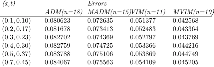
Table 1. Numerical results for Example 4.2
(x,t) Errors
ADM(n=18) MADM(n=15)VIM(n=11) MVIM(n=10) (0.1,0.10) 0.080623 0.072635 0.051377 0.042568 (0.2,0.17) 0.081678 0.073413 0.052483 0.043364 (0.3,0.23) 0.082702 0.074369 0.052797 0.043769 (0.4,0.30) 0.082759 0.074725 0.053366 0.044216 (0.5,0.37) 0.083788 0.075106 0.053869 0.044749 (0.7,0.45) 0.084067 0.075563 0.054109 0.045205
(x,t) Errors
Table 1, shows that, approximate solution of the Sawada-Kotera equation is conver-gence with 7 iterations by using the HAM . By comparing the results of Table 1 , we can observe that the HAM is more rapid convergence than the ADM, MADM, VIM, MVIM, HPM and MHPM.
5
Conclusion
The HAM has been shown to solve effectively, easily and accurately a large class of nonlin-ear problems with the approximations which are convergent are rapidly to exact solutions. In this work, the HAM has been successfully employed to obtain the approximate solution to analytical solution of the Sawada-Kotera equation. For this purpose, we showed that the HAM is more rapid convergence than the ADM, MADM, VIM, MVIM, HPM and MHPM. Also, the number of computations in HAM is less than the number of computations in ADM, MADM, VIM, MVIM, HPM and MHPM.
References
[1] C.Qu, Y. Si, R.Liu, On affine Sawada-Kotera equation, Chaos, Solitons and Fractals 15 (2003) 131-139.
[2] AM. Wazwaz, The Hirota’s direct method and the tanh-coth method for multiple-soliton solutions of the Sawada-Kotera-Ito seventh-order equation, Applied Mathe-matics and Computation 199 (2008) 133-138.
[3] A. Salas, Some solutions for a type of generalized Sawada-Kotera equation, Applied Mathematics and Computation 196 (2008) 812-817.
[4] B. Chen, Y. Xie, An auto-Backlund transformation and exact solutions of stochastic Wick-type Sawada-Kotera equations, Chaos, Solitons and Fractals 23 (2005) 243-248.
[5] AM Wazwaz, The extended tanh method for new solitons solutions for many forms of the fifth-order KdV equations, Applied Mathematics and Computation 184 (2007) 1002-1014.
[6] H.Jafari, A. Yazdani, J. Vahidi, DD. Ganji,Application of He’s Variational Iteration Method for Solving Seventh Order Sawada-Kotera Equations, Applied Mathematical Sciences 10 (2008) 471-477.
[7] C. Liu,Z. Dai, Exact soliton solutions for the fifth-order Sawada-Kotera equation, Applied Mathematics and Computation 206 (2008) 272-275.
[8] J. Zhang , J. Zhang, L. Bo, Abundant travelling wave solutions for KdV-Sawada-Kotera equation with symbolic computation, Applied Mathematics and Computation 203 (2008) 233-237.
[10] Z. Popowicz,Odd Hamiltonian structure for supersymmetric Sawada-Kotera equation, Physics Letters A 373 (2009) 3315-3323.
[11] SH. Behriy,H. Hashish, IL. E-Kalla, A. Elsaid,A new algorithm for the decomposition solution of nonlinear differential equations, App.Math.Comput. 54 (2007) 459-466.
[12] MA. Fariborzi Araghi, Sh.S. Behzadi, Solving nonlinear Volterra-Fredholm integral differential equations using the modified Adomian decomposition method, Comput. Methods in Appl. Math. 9 (2009) 1-11.
[13] AM. Wazwaz, Construction of solitary wave solution and rational solutions for the KdV equation by ADM, Chaos, Solution and fractals 12 (2001) 2283-2293.
[14] AM. Wazwaz, A first course in integral equations, WSPC, New Jersey; 1997.
[15] IL. El-Kalla, Convergence of the Adomian method applied to a class of nonlinear integral equations, Appl.Math.Comput. 21 (2008) 372-376.
[16] JH. He, XH. Wu,Exp-function method for nonlinear wave equations. Chaos, Solitons and Fractals 30 (2006) 700-708.
[17] JH. He, Variational principle for some nonlinear partial differential equations with variable cofficients, Chaos, Solitons and Fractals 19 (2004) 847-851.
[18] JH. He, Wang Shu-Qiang,Variational iteration method for solving integro-differential equations, Physics Letters A 367 (2007) 188-191.
[19] JH. He, Variational iteration method some recent results and new interpretations, J. Comp. and Appl. Math. 207 (2007) 3-17.
[20] MA. Fariborzi Araghi, Sh.S. Behzadi, Solving nonlinear Volterra-Fredholm integro-differential equations using He’s variational iteration method, International Journal of Computer Mathematics, DOI: 10.1007/s12190-010-0417-4, 2010.
[21] TA. Abassy, El-Tawil, H. El. Zoheiry,Toward a modified variational iteration method (MVIM), J. Comput. Apll. Math. 207 (2007) 137-147.
[22] TA. Abassy, El-Tawil, H. El. Zoheiry, Modified variational iteration method for Boussinesq equation, Comput. Math. Appl. 54 (2007) 955-965.
[23] SJ. Liao,Beyond Perturbation: Introduction to the Homotopy Analysis Method, Chap-man and Hall/CRC Press,Boca Raton, 2003.
[24] SJ. Liao, Notes on the homotopy analysis method: some definitions and theorems, Communication in Nonlinear Science and Numerical Simulation 14 (2009) 983-997. [25] MA. Fariborzi Araghi, Sh.S. Behzadi,Numerical solution of nonlinear
Volterra-Fredholm integro-differential equations using Homotopy analysis method, Journal of Applied Mathematics and Computing, DOI: 10.1080/00207161003770394, 2010. [26] E. Babolian, J. Saeidian, Analytic approximate solutions to Burger, Fisher, Huxley
[27] J. Biazar, H. Ghazvini, Convergence of the homotopy perturbation method for partial differential equations, Nonlinear Analysis: Real World Application 10(2009) 2633-2640.
[28] M. Ghasemi , M. Tavasoli , E. Babolian, Application of He’s homotopy perturbation method of nonlinear integro-differential equation, Appl. Math. Comput. 188 (2007) 538-548.
[29] A. Golbabai , B. Keramati, Solution of non-linear Fredholm integral equations of the first kind using modified homotopy perturbation method, Chaos Solitons and Fractals 5 (2009) 2316-2321.
[30] M. Javidi,Modified homotopy perturbation method for solving linear Fredholm integral equations, Chaos Solitons and Fractals 50 (2009) 159-165.
[31] MA. Fariborzi Araghi, SS. Behzadi, Numerical solution for solving Burger’s-Fisher equation by using Iterative Methods, Mathematical and Computational Applications, In Press, 2010.
[32] S. Abbasbandy, Modified homotopy perturbation method for nonlinear equations and comparsion with Adomian decomposition method, Appl. Math. Comput 172 (2006) 431-438.
[33] A. Yildirim, ST. Mohyud-Din, DH. Zhang, Analytical solutions to the pulsed Klein-Gordon equation using Modified Variational Iteration Method (MVIM) and Boubaker Polynomials Expansion Scheme (BPES), Computers and Mathematics with Applica-tions 59 (2010) 2473-2477.
[34] SA. Sezer, A. Yildirim, ST. Mohyud-Din, Hes homotopy perturbation method for solving the fractional KdV-Burgers-Kuramoto equation, International Journal of Nu-merical Methods for Heat and Fluid Flow 21 (2011) 448-458.
[35] AA. Yildirim, Variational iteration method for modified Camassa-Holm and Degasperis-Procesi equations, International Journal for Numerical Methods in Biomedical Engineering 26 (2010) 266-272.
[36] AA. Yildirim, Solution of BVPs for Fourth-Order Integro-Differential Equations by using Homotopy Perturbation Method, Computers and Mathematics with Applica-tions 56 (2008) 3175-3180.
[37] AA. Yildirim, The Homotopy Perturbation Method for Approximate Solution of the Modified KdV Equation, Zeitschrift fr Naturforschung A, A Journal of Physical Sci-ences 63 (2008) 621-626.
[38] AA. Yildirim,Application of the Homotopy perturbation method for the Fokker-Planck equation, International Journal for Numerical Methods in Biomedical Engineering 26 (2010) 1144-1154.
[40] Sh. S. Behzadi, MA. Fariborzi Araghi,The use of iterative methods for solving Naveir-Stokes equation, J. Appl. Math. Informatics 29 (2011) 1-15.
[41] S. Abbasbandy, Numerical method for non-linear wave and diffusion equations by the variational iteration method, Q1 Int. J. Numer. Methods Eng. 73 (2008) 1836-1843.
[42] S. Abbasbandy, A. Shirzadi,The variational iteration method for a class of eight-order boundary value differential equations, Z. Naturforsch. A 63 (2008) 745-751.