ISSN: 2333-6064 (Print), 2333-6072 (Online) Copyright © The Author(s). All Rights Reserved. Published by American Research Institute for Policy Development DOI: 10.15640/jfbm.v3n2a4 URL: http://dx.doi.org/10.15640/jfbm.v3n2a4
A Study of the Relationship between Bank Survival and Cost Efficiency
Lien-Wen Liang
1, Cheng-Ping Cheng
2& Yi-Pin Lin
3Abstract
This study aims to investigate the relationship between a bank’s survival and its cost efficiency by examining47 commercial banks in Taiwan between the years 2000 and 2008. Based on the CAMELS model, wefirst use logistic regression to extract the key factors which might affect bank survival. Then, according to Battese and Coelli (1995), we simultaneously estimate the stochastic cost frontier function and the inefficiency functionto evaluate the bank’s cost efficiency. Our main empirical findings are as follows: (1) Four key factors that cause bank survival or failure are debt ratio, non-performing loans (NPLs) ratio, growth rate of assets and bank’s ownership. (2) The higher the debt ratio and the NPL ratio, the worse is the efficiency of banks. (3) The cost efficiency of state owned banks are better than that of private banks. (4) The averagecost efficiency of failed banks is worse than that of survived banks.
Keywords: CAMELS, Logistic Model, Bank Failure, Stochastic Frontier Approach
Introduction
The banking industryin Taiwan is a “franchise industry.” The number of banks’ licenses was regulated before 1985. However, under various external and internal pressures, Taiwan’s government was forced to implement the financial liberalization policy. In 1991, Ministry of Finance, on one hand, newly set up 16 commercial banks, on the other hand, and approved the transformation of credit cooperatives, trust investment companies, and medium business banks into commercial banks. As a result, the number of banks and affiliates soared. Owing to the limited market size with high homogeneity, the substantial opening up of financial institutions resulted in excessive competition which ledsteadily falling bank interest rates, and a gradual decline in asset quality.
Following Asian financial crisis in 1997 and Taiwan’s local financial crisis in 19984, the impact of financial
crisis caused a steep climb in banks’ non-performing loans (NPLs) and poor asset quality. For example, the four years after 1998, the NPL rates of Taiwan’s banks were4.36%, 4.88%, 5.34%, and 7.48%, respectively.
The credit card debt in 2005 dealt yet another blow to Taiwan’s banking industry. Overbanking led to a continual decrease in the banks’ deposit interest rate. Moreover,the rapid expansion of credit cards and cash cards encouraged banks to float junk cards to milk the consumer finance market for profits. This resulted in huge NPLs, bad debt losses, and erosion of profits. In 2004, the overall surplus of domestic banks stood at $155.3 billion, but itfell to $78.6 billion by 2005. In 2006, losses stood at $7.4 billion. The banks suffered heavy lossesfrom the double credit card debt bubble.In a bid to bear these long-term losses, Taiwan’s banks were merged, taken over by deposit and insurance corporations, or the rights of ownership were transferred.
1 Associate Professor, Department of Banking and Finance, Chinese Culture University, Taiwan. E-mail:[email protected] 2Associate Professor, Department of Finance, National Yunlin University of Science and Technology, Taiwan. E-mail:
[email protected], corresponding author.
3Graduate Student, Soochow University, Taiwan. E-mail: [email protected]
This study aims to explore the crucial factors that affect the survival or failure of Taiwan’s banks. We also intend to compare the different impact of these factors between failed banks and surviving banks. Therefore, this study focus on the banks’ cost efficiency and survival problem.We first use a logistic regression model to determine the crucial variables affecting the survival or failure of banks. Then, based on the stochastic frontier approach proposed by Battese and Coelli(1995), we simultaneouslyestimate the banks’ cost efficiency and the impacts of the crucial characteristic factors on banks’ cost inefficiency. Finally, we discuss the relationship between the crucial factors and the survival of banks. Following introduction, section 2 reviews relevant literature. In Section 3, we discuss the methodology and data sources. Section 4 presents an analysis of the empirical results. Section 5 is a brief conclusion with policy suggestions.
2. Literature Review
2.1. Definition of bank survival
A banking crisis is usually also referred to as a “bank failure” in the existing literature. However, a few studies in Taiwan even use the term “failed bank.” It is a term that is more commonly referred to as “problematic financial institution” or a “poorly managed financial institution”. There are a number of studies focusing on the issue of failed banks. For instance, González-Hermosillo (1999) proposed that all banks that agree to receive assistance from the Federal Deposit Insurance Corporation (FDIC) should be considered as failed banks5. Later, the paper suggested that
the coverage ratio6could be used as a threshold variable in determining whether banks have failed. He suggested that
the coverage ratio of banks in normal operationsshould not be lower than 1.5. Thomson (1991) defined a bank’s economic failure as the bank’s inability to repay its debts. By statutory regulation, a bank was deemed a failure when the regulator declaredthat ithad to close down.Gajewsky(1990), Demirgüç-Kunt(1991), Leaven(1999), and Bongini, Claessens and Ferri(2001)defined distress as all those instances in which a financial institution hadreceived external support as well as when it was directly closed. Based on the previous literature, distress can be identified asone of the followings: (1) the financial institution was closed; (2) the financial institutionwas merged with another financial institution; (3) the financial institution wasrecapitalized by either the Central Bank, the Deposit Insurance Corporation, or an agencyspecifically created to tackle the crisis;(4) the financial institution’s operations weretemporarily suspended.
The usage of the term “failed banks” or “banking crisis”in the literature has the widest scope and is legally binding. In this paper, based on the definition used in the literature andin regulations, a Taiwanese bank is deemed as a failed bank if one of the following conditions are met: (1) a bank is merged with another financial institution; (2) a bank is subject to asset restructuring and takeover by Taiwan’s Financial Supervisory Commission; and (3) a bank’s management right has been transferred.
2.2. Bank survival and efficiency
In studies of bank survival, Demirgüç-Kunt and Detragiache (1997) use a multiple variablelogit model to identify the crucial factors influencing the survival of a bank. Theempirical results show that an overall sluggish economic environment is prone to banking crises. Kaminsky and Reinhart (1999) find that, problems in the banking sector typically precede a currency crisis—the currency crisis deepens the banking crisis, activating a vicious spiral; financial liberalization often precedes banking crises.
5Few people in Taiwan use the term “failed bank.” This commonly used term is “problematic financial institution” or “poorly
managed financial institution.” For the “poorly managed financial institutions,” the competent authorities, such as the Ministry of Finance, have adopted the narrowest definition, which is the “adjusted net worth in negative values,” as stipulated in Article 4 of the Financial Restructuring Fund Setup and Management Regulations. Those deemed by the competent authorities to be unable to clear their debts or to continue to operate, the authorities have not adopted them because of a lack of objective identification standards.
6The numerator of the coverage ratio is the equity and the bad debt allowance minus the overdue loans; the denominator is the
Mendis (2002) employs a multiple variablelogit model to determine the factors in a banking crisis in China with a special focus on the effects of the exchange rate system, international capital flows, and trade conditions.Bonfiglioli (2008) finds a significant association between banking crises and the stock of foreign liabilities in developed countries, but she does not find any association in developing economies.
Canbas et al.(2005) find that, through anIEWS (integrated early warning system), an early warning system is considered an effective tool for bank examination and supervision process for detection of banks, which are experiencing serious problems. Results of the study show that, if IEWS is effectively employed in bank supervision, it can be possible to avoid from the bank restructuring costs at a significant amount of rate in the long run.
The stochastic frontier analysis (SFA) is one of the most widely used approaches inanalyzing bank efficiency. Kaparakis et al. (1994), Mester (1996), and Kulasekaran and Shaffer (2002)are among those whostudyAmerican banks and find that the higher the capital adequacy of banks, the better is thebank efficiency. They also find that thehigher the proportion of construction and personal mortgage loansinthe total loan ratio, the worse thebank efficiency. Altunbas et al. (2000)and Cavallo and Rossi (2001) use Japanese and European banks as their sample, and find that technology progress is able to cut banks’ operating cost. Smallbanks in these countries had economies of scale. Therefore,while large banks areexpected to focus on diversifying products, small banks should make efforts on the expansion of product scale. Bonin et al. (2005) analyzes the effect of the shareholding structure of developing countries on bank inefficiency through stochastic frontier analysis. Its empirical results showed that the effect of state-owned and private-state-owned on bank efficiency was insignificant. In contrast, the proportion of domestic banks and foreign banks in the shareholding structure wasa significant factor influencing bank efficiency. Laeven and Levine (2009) explored the relationship between bank governance and management, and risk, and found that higher minimum capital requirements contributed to bankstability by reducing the risk of bank management. Behr et al. (2010) demonstrated that high market competition implied low bank franchising value. It also finds that capital adequacy and bank risk have a significantly negative relation.
In sum, many studies have adopted a logit approach to develop an early warning model that can predict a banking crisis so thatto control the possible risks. Some studies have used the stochastic frontier approach to evaluate banks’ efficiency. However, most studies have only adopteda single research method and have seldom take into account the possible environmental or characteristic factors which might affect the survival of a bank. Thus, this study will combine a logistic regression model withBattese and Coelli (1995)’s stochastic frontier analysis to examine the impacts of the key factors of CAMELS theory on the cost efficiency of banks.
3. Research Methods and Empirical Models
3.1. Logistic regression model
When the dependent variable is binary or of dichotomous response in nature, a logistic regression model is a power tool. The conditional probability of the occurring events is defined as,P y( i1 )xi piwhile that of the
non-occurring events is defined as1P y( i1 ) 1xi pi.The logistic regression model can be obtained as follows:
1
i
i
x
i x
e p
e
and
1 1
1 i
i x
p
e
(1)
wherepi is the probability of the occurring event.
1
i
x i
i
p e p
(2) 3.2. Stochastic frontier approach
Based on Battese and Coelli (1995), in this paper, the stochastic frontier approach takes into account environmental factors which might affect the technical inefficiency.
Based on Battese and Coelli (1995), this study specifies the following stochastic translog cost function with three inputs and three outputs, shown in the (3). In order to satisfy the condition of homogeneous of degree onein factor prices, as proposed by Allen and Rai(1996), the total cost and input factor price are divided by the labor input price for standardization. The cost function can thus be rewritten as:
2
1 3
0 1 1 2 2 3 3 1 3 11 1
2 2 2
1
ln ln ln ln ln ln (ln )
2
it it it
it it it it
it it it
TC P P
Y Y Y Y
P P P
2 2
22 2 33 3 12 1 2 13 1 3 23 2 3
1 1
(ln ) (ln ) ln ln ln ln ln ln
2 Yit 2 Yit Yit Yit Yit Yit Yit Yit
2 2
1 3 1 3 1
11 33 13 11 1
2 2 2 2 2
1 1
ln ln ln ln ln ln
2 2
it it it it it
it
it it it it it
P P P P P
Y
P P P P P
3 1 3 1
13 1 21 2 23 2 31 3
2 2 2 2
ln ln it ln ln it ln ln it ln ln it
it it it it
it it it it
P P P P
Y Y Y Y
P P P P
3 33 3 2
ln ln it
it it it
it
P
Y v u
P
(3)
Where represents total cost of the DMU. is the nth output(loans, investment,and non-interest income, respectively). is the mth input price (price of funding, labor,and capital,respectively) andi is the banking firmi.
, , , ,
are the parameters to be estimated.v
itanduit are random variables whose distribution functions are:
0, 2
~ V
it N
v ; ~ ( , 2)
u t i t i
i N m Z
u
it
u is cost inefficiency which is specified as following: 0 1 1 2 2 3 3 4 4
it it it it it it
u Z Z Z Z (4)
We select four characteristic variables that might affect the cost inefficiency of banks. Section 3.3 illustrates the detailed definitions of these variables.
3.3. Sample Data and Definitions of Variables
We use yearlydatawhich is from the report of Taiwan’s Central Bank and the data bank of Taiwan Economic Journal (TEJ). The data consists of 47 commercial banks in Taiwan between the years 2000 and 2008, which is anunbalanced panel data7. Each sample bank has durations of at least three years and might extend to nine years. Any
sample bank survived less than three years has been excluded.
7Arellano and Bond (1991) pointed out that the unbalanced panel data sample size is often larger than the balanced panel data
sample size, which can reduce the problem of self-selection bias. Moreover, there is no great disparity in the measurement method used.
it
TC Yn
m
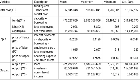
Table 1: Variable Definitions and Descriptions
Unit: thousand dollars, people, %
Variable Description Mean Maximum Minimum Std. Dev.
total cost(TC)
funding cost +labor cost + capital cost
17,945,348 108,067,841 1,202,605 18,352,137
Input
funds(X1) deposits +
borrowing 476,287,869 2,852,358,966 28,164,312 511,982,775
labor(X2) total employees 2,996 8,892 506 2,203
capital(X3) net fixed assets 11,280,744 99,076,537 696,056 14,435,396 price of funds
(P1)
interest payments / ( deposits + borrowing )
0.0266 0.1190 0.0092 0.0144
price of labor (P2)
employee salary /
total employees 1,015 2,097 213 310
price of capital (P3)
operating expense
/net fixed assets 0.3552 1.5575 0.0052 0.2364
Output
output (Y1) loans 375,232,221 1,886,393,629 7,279,023 394,806,695 output (Y2) investment 85,509,676 791,351,550 311,805 117,501,692 output (Y3) non-interest
income 2,383,732 21,237,887 16,619 3,040,638
The main variables used in our cost model are defined in Table 1. The input variables include funds(X1), labor
(X2) and capital (X3). The price of funds (P1) is the costs of funds (interest payments) divided by total deposits and
total borrowing. The price of labor (P2) is the labor costs (employee salary) divided by the total number of employees.
The price of capital (P3) is the capital costs (operating expense) divided by the net fixed assets.The output variables
consists of loans (Y1),investment (Y2) and non-interest income (Y3).
For inefficiency model, the key factors are selected based on CAMELS theory. Shen and Lin (2009) used the CAMELS indicators to measure the performance of bank privatization.Estrella et al. (2000) exploitedcapital adequacy ratio and other existing indicators to predict the failure of banks.Therefore, this study also usesfinancial ratios to identify the factors that cause a discrepancy in the operating performance ofsurvival andfailed banks. We employ a logistic regression model to choose 4 possible critical variables which might affect surviving of a bank: debt ratio, NPL ratio, asset growth rate, and ownership. The definitions and possible impacts of these four variables are explained as the following.
(1).Debt ratio: It is the ration of total debt to total assets. It can be used to measure the comprehensiveness of a bank’s financial structure and the ratio of a bank’s funds from external sources. When the external debt is too high, the leverage factors will increase the risks. If the operation falls short of expectations, the bank may be at risk of closure.
(3).Asset growth ratio: It is a ratio of thepercentage of assetchanged in assets forthe same period in the previous year. It can be used to measure whether or not the bank size has expanded. Increases in assets can result either from increases in debts or increases in equity. Therefore, the higher the asset growth rate, the better is a company’s future growth.
(4).Ownership: It is a dummy variable forstated owned and private banks. According to “Taiwan’s Article 3 of “Statute of Privatization of Government-Owned Enterprises” and “Article 11 of “Enforcement Rules of Statute of Privatization of Government-Owned Enterprises”,when the government’s stake holding in a public enterprise falls to below 50%, the enterprise will become a privately operated one. However, government often remains the largest shareholder in private companies. As a result, the designated directors and supervisors are controllers in these companies. This study defines state-owned banks and privatized public share banks as public-owned banks dominated by the government in terms of the rights to engage in bank operations and personnel.
4. Empirical Analysis
4.1. Empirical Result of Logistic Regression
A logistic regression model is used to identify the factors that affect the operational efficiency of the failed banks and surviving banks. The original possible factors include: debt ratio, capital adequacy ratio, capital adequacy ratio classes, NPL ratio, return on assets, liquid reserve ratio, asset growth rate, ownership etc. We employ backward stepwise regression to select the variables by eliminating insignificant variables one by one. The omnibus test shows that the chi-square test value is 228.164 which reaches 1% significance level. The chi-square values of the overall regression model are significant. With the failed banks and surviving banks each accounting for 50% of the critical value, the model’s overall classification accuracy rate is 88.6%. The prediction accuracy rate of the surviving banks is 96.6%, and that of the failed banks is 68.6%. The model classification is as shown in Table2.
Table 2: Percentage Correct of Logistic Regression Model
Surviving banks Failed banks Percentage Correct
Surviving banks 253* 9* 96.6**
Failed banks 33* 72* 68.6**
Overall Percentage 88.6**
Note: *denotes the number of banks, ** denotes the estimation, the unit is percentage.
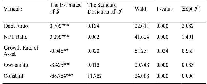
Table 3 shows the estimated parameter values and related statistics of the logistic model. The Wald test values of the debt ratio, NPL ratio, asset growth rate, andownership are all significant at the 5% level, indicating that the four variables are significantly correlated with whether or not banks survive.
Table 3: Parameter Estimation of Logistic Regression Model
Variable The Estimated of
The Standard Deviation of
Wald P-value Exp(
)Debt Ratio 0.709*** 0.124 32.611 0.000 2.032
NPL Ratio 0.399*** 0.062 41.624 0.000 1.491
Growth Rate of
Asset -0.046** 0.020 5.123 0.024 0.955
Ownership -3.425*** 0.618 30.743 0.000 0.033
Constant -68.764*** 11.782 34.063 0.000 0.000
Based on Battese and Coelli (1995), we use the maximum likelihood method to estimate the cost model and inefficiency model. The result is showed in Table 4. We use the likelihood ratio (LR) test to determine whether the proposed inefficiency model is appropriate, as given below:
0 1
2 ln ln
LR L H L H (5)
whereln
L
H0
is log-likelihood function value of the restricted model and ln
L
H1
is the one for the unrestricted model. Our LR test statistic is 111.6506 (greater than 2
0.01 6 16.81
), which rejectsH0at the1% significance level andimplies the suitability of the proposed inefficiency model.
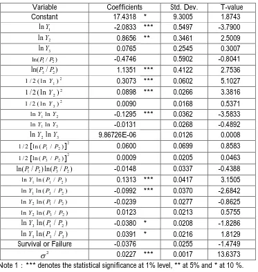
Table 4 shows the estimated results of the stochastic frontier cost function. We add a survival dummy variable to the explanatory variables of the cost function, to distinguish the merits and demerits of bank operations. With 0 representing surviving banks and 1, the failed banks.
Table 4: Empirical Results of the Stochastic Cost Function
Variable Coefficients Std. Dev. T-value
Constant 17.4318 * 9.3005 1.8743
1
lnY -2.0833 *** 0.5497 -3.7900
2
lnY 0.8656 ** 0.3461 2.5009
3
lnY 0.0765 0.2545 0.3007
1 2
ln(P P/ ) -0.4746 0.5902 -0.8041
3 2
ln(P /P) 1.1351 *** 0.4122 2.7536
2 1
1 / 2 ( l n Y ) 0.3073 *** 0.0602 5.1027
2 2
1 /2 ( lnY ) 0.0898 *** 0.0266 3.3816
2 3
1 / 2 ( l n Y ) 0.0090 0.0168 0.5371
1 2
lnY lnY -0.1295 *** 0.0362 -3.5833
1 3
lnY lnY -0.0131 0.0268 -0.4892
2 3
lnY lnY 9.86726E-06 0.0126 0.0008
21 2
1 / 2 l n (P / P ) 0.0600 0.0699 0.8583
23 2
1 / 2 ln (P / P ) 0.0009 0.0205 0.0463
1 2 3 2
ln(P/P) ln(P /P) -0.0148 0.0337 -0.4388
1 1 2
lnY ln (P / P ) 0.1313 *** 0.0417 3.1505
1 3 2
lnY ln (P /P ) -0.0992 *** 0.0370 -2.6842
2 1 2
lnY ln (P /P ) -0.0239 0.0277 -0.8625
2 3 2
lnY ln (P /P ) 0.0123 0.0213 0.5755
3 1 2
lnY ln (P /P ) -0.0380 * 0.0208 -1.8286
3 3 2
lnY ln (P /P ) 0.0391 * 0.0216 1.8129
Survival or Failure -0.0376 0.0255 -1.4749
2
0.0227 *** 0.0017 13.6373Note 1:*** denotes the statistical significance at 1% level, ** at 5% and * at 10 %. Note 2:Y1 is loan, Y2 is investment, Y3 is non-interest income, P1 is price of funds,
The Wald test results show that the banks’ loans (Y1), investments (Y2), and non-interest income (Y3) are significantly positive related to total cost (TC), which satisfy the condition of homogeneity of cost function. The fund price (P1), labor price (P2), and capital price (P3) are also significantly positive related to total cost, which are consistent with the condition of non-decreasing of factor prices of a cost function.
In addition, every cost function has to meet the regularity conditions8. The aforementioned Wald chi-square
test confirmed that the cost function is the non-decreasing function of prices. Using the homogeneous of degree one,9we examine the factor share function to obtain the cost function and the factor price first derivative, as expressed
below: 3 3 * 1 1 ln 1 ln ln ln 2
j j ij i ij i
i i
j
TC
S P Y
P
(6)where *
j
S lies between 0 and 1, and the total of the factor shares is 1. Our results show that the banks’ fund shares, labor shares, and capital shares are positively and significantly correlated with total cost. The sum of the three factor shares’ estimated equals 1.
The Hessian matrix is used to examine whether the cost function is a concave function of factor prices meaning the second-order partial differential equation of factor prices forms a negative semi-definite matrix10. The
results show that the second-order results H1 is significantly less than 0, and H2 is significantly greater than 0. Although H3is greater than 0, it is not significant. This finding coincides with the characteristics of the concave function of factor prices.
In sum, the cost functions estimated indeed meet the regularity conditions of economic theory. 4.3. Empirical Result of Inefficiency Model
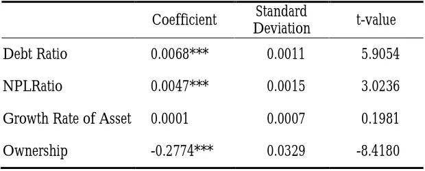
Table5 shows the estimated results of the inefficiency model. The relation between the inefficiency variables and cost inefficiency are described as follows:
8The formal conditions proposed by Varian (1992) are: (1) the cost function is the non-decreasing function of factor prices, (2)
the cost function is the homogeneous first-order of factor prices, (3) the cost function is the concave function of factor prices, and (4 ) the cost function and factor pricesare a function of the continuous second derivative.
9According to the equation 3, the homogeneous first-order conditions are: 3
1 1 j j
, 3 1 0 ij i
, 3 1 0 ij i
.10The third-order of the Hessian matrix is defined as: *
1 11 0 H C ,
* *
11 12
2 * *
21 22 0 C C H C C , * * *
11 1 2 13
* * *
3 2 1 22 2 3
* * *
31 3 2 33
0
C C C
H C C C
C C C
,
where, * 2 *
/
ij i j
Table 5: The Empirical Results of Inefficiency
Coefficient Standard
Deviation t-value
Debt Ratio 0.0068*** 0.0011 5.9054
NPLRatio 0.0047*** 0.0015 3.0236
Growth Rate of Asset 0.0001 0.0007 0.1981
Ownership -0.2774*** 0.0329 -8.4180
*** denotes the statistical significance at 1% level, ** at 5% and * at 10 %.
(1) The effects of the debt ratio on banks’ cost inefficiency are significantly positive, indicating that the higher the debt ratio would reduce then cost efficiency of a bank. Since a high debt ratio means the bank is heavily rely on external funds, the bank thus would be poor to repay debts. Finally, the cost efficiency will be worse.
(2) The effects of the NPL ratio on banks’ cost inefficiency are also significantly positive and, indicating that the higher the NPL ratio, the greater is the uncollectable bad debt, and thus the poorer the asset quality (Hughes and Mester, 1993; Berger and De Young, 1997; Drake and Hall, 2003). This, in turn, results in banks’ reduced profits, increased operating risks, and diminished cost efficiency.
(3) The asset growth rate has a positive effect on banks’ cost inefficiency, indicating that, despite the banks’ profitable gains at the time of asset or scale expansion or increases in loans, the costs will also increase. However, this study found that such an increase is not significant. In particular, the failed banks often increase the risk-weighted loans for the sake of survival, which results in added costs and operational inefficiency.
(4) The effects of ownership (stateorprivately-owned banks) on cost inefficiency is significantly negative, which shows that in face of a financial crisis, stated owned banks are better trusted by the people. In Taiwan, government usually guarantee the safety of deposits for state owned banks, private banks thus often encounter loss when faced with bank runs or a financial crisis. In addition, state owned banks are relatively easy to increase their cost efficiency because they have more stable client sources and more funds (Bhattacharyya et al. 1997).
4.4. Rank of cost efficiency
Table 6: Rank of Cost Efficiency of Failed Banks from 2000 to 2008
Bank Maximum Minimum Mean Standard
Deviation Rank
Farmers Bank of China 2.0327 1.8784 1.9566 0.0718 1
Yuanta Commercial Bank 2.4681 2.3029 2.3616 0.0592 2
Lucky Bank 2.4981 2.2142 2.3695 0.1191 3
Kao Shin Commercial Bank 2.5473 2.2960 2.4405 0.1055 4
Grand Commercial Bank 2.5268 2.4560 2.4862 0.0365 5
Kings Town Bank 2.6157 2.2902 2.4991 0.1317 6
Chinese Bank 2.9799 2.3078 2.5133 0.2175 7
Hsinchu International Bank 2.6933 2.4408 2.5302 0.0874 8
Taitung Business Bank 2.7561 2.4167 2.5500 0.1130 9
Jih Sun International Bank 2.7228 2.5295 2.5722 0.0580 10
Bowa Bank 3.3032 2.4142 2.7024 0.2615 11
Bank of Overseas Chinese 2.9151 2.5795 2.7048 0.1365 12 Enterise Bank of Hualien 2.9641 2.5682 2.7690 0.1572 13 Chinfon Commercial Bank 3.6522 2.4994 2.8247 0.3498 14 Kaohsiung Business Bank 3.6534 2.7676 3.2515 0.3746 15
Chung Shing Bank 5.8045 2.9302 4.1576 1.1395 16
Mean of Cost Efficiency 2.6681
Table 7: Rank Cost Efficiency of Surviving Banks from 2000 to 2008
Bank Maximum Minimum Mean Standard
Deviation Rank
Chiao Tung Bank 1.5468 1.4500 1.4969 0.0315 1
Mega International Commercial Bank 1.9045 1.6550 1.7505 0.0817 2
Land Bank of Taiwan 1.9017 1.7103 1.7898 0.0674 3
Taiwan Cooperative Bank 1.9048 1.6993 1.8165 0.0697 4
Bank of Kaohsiung 1.9408 1.7584 1.8566 0.0687 5
Bank of Taiwan 2.0511 1.7424 1.9181 0.0910 6
Taiwan Business Bank 1.9860 1.8597 1.9346 0.0441 7
Chang Hwa Commercial Bank 2.0437 1.8715 1.9463 0.0592 8
Hua Nan Commercial Bank 2.0386 1.8752 1.9511 0.0530 9
First Commercial Bank 2.0959 1.8348 1.9626 0.0903 10
Taipei Fubon Commercial Bank 2.4434 2.0355 2.2428 0.1588 11
International Bank of Taipei 2.3388 2.1954 2.2540 0.0609 12
Far Eastern InternationalBank 2.3349 2.1293 2.2598 0.0712 13
Cota Bank 2.3869 2.2106 2.2792 0.0602 14
Entie Commercial Bank 2.3606 2.2290 2.2957 0.0542 15
The Shanghai Commercial and Savings Bank 2.3819 2.2131 2.3053 0.0639 16
Cathay United Bank 2.3846 2.2926 2.3359 0.0330 17
Bank Sinopac Company Limited 2.5862 2.0753 2.3451 0.1594 18
Hwatai Bank 2.4174 2.2565 2.3477 0.0592 19
E.Sun Commercial Bank 2.4842 2.2794 2.3886 0.0653 20
Fubon Commercial Bank 2.4802 2.3008 2.4007 0.0707 21
Ta Chong Bank 2.4971 2.2957 2.4023 0.0750 22
Cathy United Bank 2.5491 2.3878 2.4564 0.0833 23
Bank of Panhsin 2.5232 2.3979 2.4593 0.0508 24
Taichung Commercial Bank 2.6280 2.3991 2.5161 0.0813 25
Chinatrust Commercial Bank 2.7571 2.3565 2.5251 0.1160 26
Union Bank of Taiwan 2.7609 2.3785 2.5636 0.1443 27
Sunny Bank 2.6367 2.5044 2.5696 0.0457 28
Taishin International Bank 2.7597 2.4676 2.5811 0.0944 29
Cosmos Bank, Taiwan 2.9845 2.5496 2.7407 0.1580 30
Taiwan Shin Kong Commercial Bank 2.9255 2.4745 2.7618 0.1590 31
Over All Mean of Cost Efficiency 2.2404
In this paper, the cost efficiency values range between 1 and
. The lower value means better performance in
cost efficiency. Figure1 shows that the average cost efficiency performances of surviving banks are all better than that of failed banks from 2000 to 2008. Some evidences in Taiwan are supporting this results. (1) Under Taiwan’s local financial crisis since 1998, the banks’NPL ratio was gradually increases. In 2001, it reached 7.48%, and the cost inefficiency increased as a result. In 2005, the Chung Shing Bank and the Kaohsiung Business Bank merged, resulting in reduced cost efficiency values. (2) In 2005, Taiwan’s credit card debt crisis also cut down the failed banks’ cost efficiency.Figure1: Average Cost Efficiency of All Banks
5. Conclusion
Following the deregulation of Taiwan’s financial sector in 1990s, Taiwan has experienced a rapid increase in the number of banks. Bank investments and financial businesses have been active. However, the overall size of Taiwan’s financial market has not expanded dramatically. As a result, the increase of the number of financial institutionsleads to excessive competition which eventually causes some banks survived andsome failed. By a logistic model, we identify four crucial factors influencing bank survival or failure. They were the debt ratio, the NPL ratio, the asset growth rate, and ownership. The four variables are found to have an accuracy rate of 96.6% in predicting the survival of banks, and an accuracy rate of 68.6% in predicting bank failures. The overall classification accuracy rate of the model is 88.6%, and the prediction accuracy rates of the variables all reach over 60%, indicating the variables possessed explanatory power. These indexes justify the use of the four variables in predicting banks’ survival or failure.
By empirical results of the inefficiency model, we find three of four key factors derived from CAMELs are directly and deeply influence the cost efficiency of Taiwan’s banks. (1) The higher the debt ratio, the worse of cost performance. Since the higher the debt ratio means the greater thereliance on external funds, the greater are the risks involved.(2) ThehigherNPLratio increases bank’s cost inefficiency. Since banks with high NPL ratio are always involved high bad loans which would lead to operational inefficiency.(3) Stated owned banks have a better performance in cost efficiency. When faced with a financial crisis, state owned banks are better trusted by the people due to government’s unlimited support.
Practically, we find that the four key factors derived from CAMELs are also heavily affect the surviving or failed of Taiwan’s banks. For the surviving banks, their financial conditions are relatively steady, the NPL ratios are maintained at below 5%, the asset quality is good, and the debt ratio and asset growth rate are maintained at a certain level. For the failed banks, their NPL ratios usually are relatively high, indicating poor asset quality. They also have high debt ratios and high financial leverage resulted in greater risks and made banking crisis more likely.
We also find mostsmall-and-medium-scale private banks taken over by Taiwan’s Central Deposit Insurance Corporation mostly are poorly managed and with high risk to fail while stated owned banks are never with this kind of crisis.
Reference
Aigner, D. J., Lovell, C. A. K., and Schmidt, P. (1977). Formulation and Estimation of Stochastic Frontier Production Function Models.Journal of Econometrics, 6(1), 21-37.
Allen, L.,and Rai, A. (1996). Operational Efficiency in Banking: An International Comparison.Journal of Banking and
Finance, 20(4), 655-672.
Altunbas, Y., Liu, M. H., Molyneux, P., and Seth,R.(2000). Efficiency and Risk in Japanese Banking.Journal of Banking
and Finance, 24(10), 1605-1628.
-0.50 1.00 1.50 2.00 2.50 3.00 3.50
2000 2001 2002 2003 2004 2005 2006 2007 2008 Year CE
Arellano, M.,and Bond, S. (1991). Some Tests of Specification for Panel Data: Monte Carlo Evidence and an Application to Employment Equations.The Review of Economic Studies, 58(2), 277-297.
Battese, G. E.,and Coelli, T. J. (1995).A Model for Technical Inefficiency Effects in A Stochastic Frontier Production Function for Panel Data.Empirical Economics, 20(2), 325-332.
Berger, A. N.,and DeYoung, R. (1997). Problem Loans and Cost Efficiency in Commercial Banks.Journal of Banking
and Finance, 21(6), 849-870.
Bhattacharyya, A., Lovell, C. A. K.,and Sahay, P. (1997). The Impact of Liberalization on the Productive Efficiency of Indian Commercial Banks.European Journal of Operational Research, 98(2), 332-345.
Bonfiglioli, A. (2008). Financial integration, productivity and capital accumulation. Journal of International Economics, 76 (2), 337–355.
Bongini, P., Claessens,S.,andFerri, G. (2001). The Political Economy of Distress in East Asian Financial Institutions.Journal of Financial Services Research, 19(1), 5-25.
Canbas, S.,Cabuk, A.,and Kilic, S. B. (2005), Prediction of Commercial Bank Failure via Multivariate Statistical Analysis of Financial Structures: The Turkish Case.European Journal of Operational Research, 166(2), 528-546. Cavallo, L.,and Rossi,S. P.S. (2001). Scale and Scope Economies in the European Banking Systems.Journal of
Multinational Financial Management, 11(4-5), 515-531.
Chiu, Y. H.,and Chen, Y. C. (2004).A Study of Banking Efficiency and Market Power. Asia-Pacific Economic and
Management Review, 8(1), 49-65.
Demirgűç-Kunt, A. (1991). On the Evaluation of Deposit Institutions.Federal Reserve Bank of Cleveland, Working Paper
No. 9104.
Demirgűç-Kunt, A.,and Detragiache, E. (1997). The Determinants of Banking Crises: Evidence from Developed and
Developing Countries.IMF Working Paper No. 106.
Drake, L.,and Hall, M. J. B. (2003). Efficiency in Japanese Banking: An Empirical Analysis.Journal of Banking and
Finance,27(5), 891-917.
Estrella, A., Park,S.,and Peristiani, S. (2000). Capital Ratios as Predictors of Bank Failure.Economic Policy Review-Federal
Reserve Bank of New York, 6(2), 33-52.
Gajewsky, G. R. (1990). Modeling Bank Closures in the 1980’s: the Roles of Regulatory Behavior, Farm Lending and the Local Economy.Research in Financial Services: Private and Public Policy 2.
González-Hermosillo, B. (1999). Determinants of Ex-Ante Banking System Distress: A Macro-Micro Empirical Exploration of Some Recent Episodes. IMF Working Paper No. 99/33.
Hughes, J. P.,and Mester, L. J. (1993). A Quality and Risk-Adjusted Cost Function for Banks: Evidence on the Too-Big-Fail Doctrine.Journal of Productivity Analysis, 4(3), 293-315.
Kaminsky, G. L.,and Reinhart, C. M. (1999). The Twin Crises: the Causes of Banking and Balance-of-Payments Problems.The American Economic Review, 89(3), 473-500.
Kaparakis, E. I.,Miller,S. M.,and Noulas,A. G.(1994). Short-Run Cost Inefficiency of Commercial Banks: A Flexible Stochastic Frontier Approach.Journal of Money, Credit, and Banking, 26, 875-893.
Kulasekaran, S.,andShaffer, S.(2002). Cost Efficiency among Credit Card Banks.Journal of Economics and Business, 54(6), 595-614.
Leaven, L. (1999). Risk and Efficiency in East Asian Banks.The World Bank Working Paper No. 2255.
Meeusen, W.,and Broeck, J. van den (1977). Efficiency Estimation from Cobb-Douglas Production Function with Composed Error.International Economic Review, 18(2), 435-444.
Mendis, C. (2002). External Shocks and Banking Crises in Developing Countries: Does the Exchange Rate Regime Matter.CESifo Working Paper No. 759.
Mester, L. J. (1996). A Study of Bank Efficiency Taking into Account Risk-preferences. Journal of Banking and Finance, 20(6), 1025-1045.
Shen, C. H.,and Lin, C. Y. (2009). The Performance of Bank Privatization: the Application of the Matching Theory.
Academia Economic Papers, 37(3), 369-405.
Thomson, J. B. (1991). Predicting Bank Failures in the 1980s.Economic Review-Federal Reserve Bank of Cleveland, 27(1), 9-20.