Vol. 9, No. 1, 2017 Article ID IJIM-00871, 15 pages Research Article
A new weighting approach to Non-Parametric composite indices
compared with principal components analysis
M. Rahimpoor ∗†, A. Heshmati ‡, A. Ahmadizad §
Received Date: 2014-01-02 Revised Date: 2015-11-03 Accepted Date: 2016-07-02
————————————————————————————————–
Abstract
Introduction of Human Development Index (HDI) by UNDP in early 1990 followed a surge in use of non-parametric and parametric indices for measurement and comparison of countries performance in development, globalization, competition, well-being and etc. The HDI is a composite index of three indicators. Its components are to reflect three major dimensions of human development: longevity, knowledge and access to resources represented by GDP per capita, educational attainment and life expectancy. In recent years additional gender and poverty aspects are included. A known example of the non-parametric index is the HDI, while Principal Components Analysis (PCA) and Factor Analysis (FA) are among the parametric counterparts. The indices differ mainly in respect to weighting the indicators in their aggregation. The non-parametric index assumes the weights, while the parametric approach estimates them. In this research, it is aimed to purpose a new weighting approach to non-parametric indices when they are used simultaneous with principal components analysis.
Keywords: Principal Components Analysis; Non-Parametric Indicators; Composite Indices; Weighting Schemes.
—————————————————————————————————–
1
Introduction
P
Ctransforms an original set of variables intoA is a statistical technique that linearly a substantially smaller set of uncorrelated vari-ables that represents most of the information in the original set of variables. Its goal is to re-duce the dimensionality of the original data set. A small set of uncorrelated variables (factors or components) is much easier to understand and use in further analysis than a large set ofcorre-∗Corresponding author. [email protected] †Department of Industrial Engineering, Kharazmi Uni-versity, Tehran, Iran.
‡Department of of Economics, Sogang University, Seoul, Korea.
§Department of Systems Management, University of Kurdistan, Sanandaj, Iran.
lated variables. The idea was originally conceived by Pearson [13] and later independently devel-oped by Hotelling [8]. The advantage in reducing the dimensions is ranking the units of comparison in a unique way avoiding contradictions in units performance ranking.
The goal of PCA is similar to FA in that both techniques try to explain part of the variation in a set of observed variables on the basis of a few underlying dimensions. However, there are important differences between the two tech-niques. Briefly, PCA has no underlying statistical model of the observed variables on the basis of the maximum variance properties of principal compo-nents. Factor analysis, on the other hand, has an underlying statistical model that partitions the total variance into common and unique variance and focuses on explaining the common variance,
rather than the total variance, in the observed variables on the basis of a relatively few underly-ing factors. PCA is also similar to other multi-variate procedures such as discriminant analysis and canonical correlation analysis in that they all involve linear combinations of correlated variables whose variable weights in the linear combination are derived on the basis of maximizing some sta-tistical property. It has been seen that princi-pal components maximize the variance accounted for in the original variables. Linear discriminant function analysis, focusing on differences among groups, determines the weights for a linear com-posite that maximizes the between group relative to within group variance on that linear composite. Canonical correlation analysis, focusing on the re-lationships between two variables sets, derives a linear composite from each variable set such that the correlation between the two derived compos-ites is maximized. For a detailed explanation see Basilevsky [3].
2
Review of the Literature
In several studies, common factor analysis (CFA) and PCA are used in either the computation of an index or to reduce several variables into fewer di-mensions. While some researchers prefer the CFA approach, a majority prefer the PCA method. For instance using several indications of economic integration and international interaction, Ander-sen and Herbertsson [1] used a multivariate factor analysis technique to compute an openness index based on trade for 23 OECD countries using sev-eral indications of economic integration and in-ternational integration. Analyzing the relation-ship between economic factors, such as income inequality and poverty, Heshmati [5] used PCA to addressing the measurement of two indices of globalization and their impacts on poverty rate and income inequality reductions. Heshmati and Oh [6] compared two indices: the Lisbon Devel-opment Strategy Index and another index cal-culated by the PCA method. They found that despite differences in ranking countries between those two indices, the United States surpassed almost all EU-member states. Also, Heshmati et al [7] estimated two forms of parametric index using PCA. The first model used a pool of all indicators without classification of the indicators by type of well-being, while the second model
es-timated first the sub-components separately and then used the share of variance explained by each principal component to compute the weighted av-erage of each component and their aggregation into an index of overall child well-being in high income countries. The method has the advantage that it utilizes all information about well-being embedded in the indicators. As mentioned above, the PCA is preferred by majority of researchers than the CFA. The CFA can be used to sepa-rate variance into two uncorrelated components. Therefore for those computing indices that relay on the common similarity over components, the PCA method might be better alternative than the CFA technique. Lim and Nguyen [12] com-pared the weighting schemes in traditional, prin-cipal component and dynamic factor approaches to summarizing information from a number of component variables. They determined that, the traditional way has been to select a set of vari-ables and then to sum them into one overall in-dex using weights that are inversely related to the variations in the components. Moreover, they founded that, recent approaches, such as the dy-namic principal component and the dydy-namic fac-tor approaches, use more sophisticated statistical and econometric techniques to extract the index. They proposed a simple way to recast the dy-namic factor index into a weighted average form.
3
Theoretical Foundations
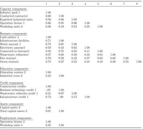
compo-Table 1: Pearson correlation matrix of infrastructure components (n=31).
1 2 3 4 5 6 7 8
Capacity component:
Industry park 1 1.00
Conducted contracts1 0.60 1.00
Exploited industrial units 0.59 0.98 1.00
Operation license 1 0.66 0.95 0.96 1.00
Workshop units 3 0.36 0.19 0.24 0.35 1.00
Resource component:
Land surface 4 1.00
Infrastructure facilities 0.71 1.00
Water amount 1 0.75 0.65 1.00
Electricity amount1 0.58 0.42 0.62 1.00
Connected to internet1 0.50 0.75 0.25 0.11 1.00
Wastewater refineries1 0.57 0.68 0.48 0.42 0.64 1.00
Fire station1 0.76 0.59 0.43 0.27 0.63 0.60 1.00
Green station1 0.75 0.37 0.52 0.45 0.16 0.39 0.55 1.00
Education component:
Education courses 2 1.00
Industrial tours 2 0.82 1.00
Credit component:
Construction credits 1.00
Business technology credit 1 -.05 1.00
Wastewater refineries credit 1 0.21 0.07 1.00
Infrastructure credit 1 0.72 -.08 0.15 1.00
Assets component:
Capital assets 2 1.00
Total capital assets 2 0.01 1.00
Employment component:
Operation license 2 1.00
Workshop units 5 0.35 1.00
Table 2: Correlation matrix of DII sub-indexes.
Capacity Resource Education Credit Assets Employment DII Capacity 1.000
Resource 0.888 1.000
Education 0.723 0.809 1.000
Credit 0.394 0.427 0.323 1.000
Assets 0.056 -0.036 -0.210 0.169 1.000
Employment 0.874 0.768 0.727 0.437 0.103 1.000
DII 0.912 0.898 0.794 0.611 0.228 0.902 1.000
nents to visually examine relative to the original variables. PCA searches for a few uncorrelated linear combinations of the original variables that capture most of the information in the original variables. We construct linear composites
Table 3: Eigenvalues of correlation matrix, n=31.
Principal Component Eigenvalue Difference Proportion Cumulative
1 10.9472502 7.8728901 0.4760 0.4760
2 3.0743601 1.3720595 0.1337 0.6096
3 1.7023006 0.1858589 0.0740 0.6836
4 1.5164417 0.1858993 0.0659 0.7496
5 1.3305425 0.1703744 0.0578 0.8074
6 1.1601681 0.2428082 0.0504 0.8579
7 0.9173599 0.3771149 0.0399 0.8978
8 0.5402451 0.0235 0.9212
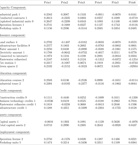
Table 4: Eigenvectors by sub-index, n=31.
Prin1 Prin2 Prin3 Prin4 Prin5 Prin6 Capacity Component:
Industrial park 1 0.2583 0.2087 0.1533 -0.0911 -0.0670 0.0161 Conducted contracts 1 0.2613 -0.2335 0.0303 0.0357 0.1089 -0.0718 Exploited industrial units 9 0.2647 -0.2209 0.0343 0.1093 0.1100 -0.1089 Operation licenses 1 0.2741 -0.1688 0.0227 0.1127 0.1743 -0.0116 Workshop units 3 0.1156 0.2596 -0.3144 0.3565 0.3354 0.0485
Resource component:
Land surface 4 0.2792 -0.1407 -0.0182 -0.0033 -0.0078 0.0555 Infrastructure facilities 9 0.2577 0.1803 0.2002 -0.0783 -0.0802 0.0001 Water amount 1 0.2250 0.0438 -0.0890 -0.3588 -0.1061 0.1575 Electricity amount 1 0.1788 -0.0642 -0.0732 -0.4017 0.3511 0.0776 Connected to internet1 0.1972 0.1216 0.4198 0.2891 -0.0844 0.0504 Wastewater refineries1 0.2187 0.0452 0.2124 -0.1312 -0.0372 -0.1254 Fire station 1 0.2317 -0.1087 0.0674 0.1919 -0.2931 -0.0733 Green spaces 2 0.2192 -0.2152 -0.3523 0.0672 0.0435 -.02934
Education component:
Education courses 2 0.2503 0.0136 -0.2526 0.0998 -0.1651 -0.0114 Industrial tours 2 0.2394 -0.0192 -0.2377 -0.3116 -0.1863 0.0044
Credit component:
Construction credits 9 0.1111 0.4440 0.0252 -0.1699 0.1011 -0.1338 Business technology credits 1 -0.0536 0.0419 0.0525 -0.0188 0.2962 0.7916 Wastewater refineries credit 1 0.1818 -0.0238 0.3668 -0.0813 0.2046 0.1596 Infrastructure credit 1 0.1288 0.4351 -0.1699 -0.2204 -0.1735 0.0128
Assets component:
Capital assets 1 -0.0616 0.1303 0.1091 -0.1129 0.5626 -0.4976 Total capital assets 2 0.0710 0.2990 0.2305 0.2643 -0.0928 0.0437
Employment component:
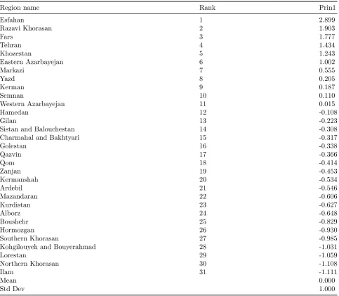
Table 5: Principal components and their aggregate index.
Region name Rank Prin1
Esfahan 1 2.899
Razavi Khorasan 2 1.903
Fars 3 1.777
Tehran 4 1.434
Khozestan 5 1.243
Eastern Azarbayejan 6 1.002
Markazi 7 0.555
Yazd 8 0.205
Kerman 9 0.187
Semnan 10 0.110
Western Azarbayejan 11 0.015
Hamedan 12 -0.108
Gilan 13 -0.223
Sistan and Balouchestan 14 -0.308
Charmahal and Bakhtyari 15 -0.317
Golestan 16 -0.338
Qazvin 17 -0.366
Qom 18 -0.414
Zanjan 19 -0.453
Kermanshah 20 -0.534
Ardebil 21 -0.546
Mazandaran 22 -0.606
Kurdistan 23 -0.627
Alborz 24 -0.648
Boushehr 25 -0.829
Hormozgan 26 -0.930
Southern Khorasan 27 -0.985
Kohgilouyeh and Bouyerahmad 28 -1.031
Lorestan 29 -1.059
Northern Khorasan 30 -1.108
Ilam 31 -1.111
Mean 0.000
Std Dev 1.000
a set of p socio-economic status indicators such as occupational level, educational level and in-come, which can be characterized as a p dimen-sional random vector (x1, x2, , xn), can be linearly transformed by y = a1x1+a2x2+? +apxp into a one dimensional index, y. In PCA, the weights (i.e.,a1, a2, ..., ap) are mathematically determined to maximize the explained variation of the linear composite or, equivalently, to maximize the sum of the squared correlations of principal compo-nent with the original variables. The linear com-posites (principal components) are ordered with respect to their variation explanation so that the first few account for most of the variation present in the original variables, or equivalently, the first few principal components together have, over all, the highest possible squared multiple correlations
Table 6: Mean value of DII and rank number.
Province Capacity Resource Education Credit
Rank Mean Rank Mean Rank Mean Rank Mean Esfahan 1 0.831 1 0.797 3 0.648 10 0.349 Razavi Khorasan 4 0.534 3 0.581 1 0.890 8 0.431 Khouzestan 5 0.522 7 0.455 6 0.292 1 0.647 East Azarbayejan 2 0.584 6 0.471 12 0.190 4 0.542
Fars 6 0.443 2 0.664 2 0.743 5 0.538
Tehran 3 0.579 4 0.572 5 0.315 23 0.201
Mazandaran 9 0.326 6 0.471 24 0.049 7 0.492 Semnan 8 0.327 10 0.301 10 0.233 12 0.325 Markazi 11 0.280 5 0.490 4 0.319 28 0.120 West Azarbayejan 12 0.268 16 0.231 8 0.265 13 0.302
Yazd 14 0.229 9 0.337 13 0.183 6 0.516
Kerman 10 0.288 8 0.339 15 0.169 20 0.223 Gilan 16 0.206 14 0.247 18 0.096 3 0.560 Golestan 22 0.131 15 0.235 16 0.159 8 0.417 Kermanshah 21 0.149 19 0.167 19 0.117 2 0.638 Hamedan 18 0.186 11 0.260 7 0.279 11 0.332 Qazvin 21 0.146 13 0.250 9 0.261 15 0.277 Sistan and Balouchestan 7 0.333 22 0.136 18 0.122 16 0.270 Kurdistan 13 0.255 24 0.094 20 0.087 19 0.253 Zanjan 17 0.195 17 0.189 14 0.170 18 0.259 North Khorasan 28 0.041 30 0.044 22 0.063 21 0.220
Qom 15 0.227 20 0.151 11 0.205 27 0.130
Boushehr 24 0.069 23 0.127 26 0.031 25 0.148 Ardebil 17 0.195 18 0.177 21 0.075 24 0.186 Charmahal and Bakhtyari 19 0.185 12 0.253 17 0.125 30 0.081 Alborz 20 0.153 21 0.144 23 0.061 31 0.065 Lorestan 27 0.052 29 0.064 30 0.002 22 0.217 South Khorasan 25 0.061 25 0.087 29 0.008 14 0.297 Ilam 29 0.038 27 0.073 28 0.014 17 0.264 Hormozgan 23 0.102 26 0.083 27 0.023 26 0.131 Kohgilouyeh and Bouyerahmad 26 0.056 28 0.067 25 0.040 29 0.097
Mean 0.258 0.276 0.201 0.307
Std Dev 0.190 0.197 0.211 0.167
are linear dependencies among the variables. If all possible principal components are used, then they define a space which has the same dimension as the variable space and, hence, completely ac-count for the variation in the variables. However, there is no advantage in retaining all of the prin-cipal components since we would have as many components as variables and, thus, would not have simplified matters. Algebraically, the first principal component, is a linear combination of
x1, x2, ..., xp, written as:
y1 =a11x1+a12x2+...+a1pxp = p ∑
i=1
a1ixi (3.1)
such that the variance of y1 is maximized given
the constraint that the sum of the squared
weights is equal to one (i.e., ∑pi=1a21i = 1). As we shall see, the random variables, xi, can be either deviation from mean scores or stan-dardized scores. If the variance of y1 is
maxi-mized, then so is the sum of the squared correla-tions ofy1with the original variablesx1, x2, ..., xp (i.e., ∑pi=1r2yrxi ). PCA finds the optimal weight vector (a11, a12, ..., a1p) and the associated variance of y1. The second principal
compo-nent, y2, involves finding a second weight vector
(a21, a22, ..., a2p) such that the variance of
y2 =a21x1+a22x2+...+a2pxp = p ∑
i=1
a2ixi (3.2)
Continue Table 7
Employment Assets DII
Rank Mean Rank Mean Rank Mean
Esfahan 3 0.542 13 0.126 1 3.293
Razavi Khorasan 1 0.787 17 0.000 2 3.222
Khouzestan 2 0.559 2 0.500 3 2.975
East Azarbayejan 4 0.474 1 0.604 4 2.865
Fars 10 0.175 17 0.000 5 2.562
Tehran 5 0.367 17 0.000 6 2.033
Mazandaran 7 0.241 8 0.227 7 1.806
Semnan 6 0.310 17 0.000 8 1.496
Markazi 8 0.196 14 0.055 9 1.460
West Azarbayejan 16 0.149 7 0.234 10 1.448
Yazd 9 0.181 17 0.000 11 1.447
Kerman 14 0.160 12 0.143 12 0.321
Gilan 17 0.140 15 0.035 13 1.284
Golestan 23 0.081 6 0.249 14 1.272
Kermanshah 20 0.114 17 0.000 15 1.184
Hamedan 24 0.064 17 0.000 16 1.121
Qazvin 19 0.128 17 0.000 17 1.062
Sistan and Balouchestan 13 0.162 17 0.000 18 1.023
Kurdistan 15 0.151 11 0.154 19 0.994
Zanjan 18 0.132 17 0.000 20 0.944
North Khorasan 25 0.038 4 0.488 21 0.893
Qom 11 0.174 17 0.000 22 0.887
Boushehr 26 0.023 3 0.489 23 0.886
Ardebil 12 0.174 15 0.000 24 0.807
Charmahal and Bakhtyari 21 0.107 16 0.007 25 0.758
Alborz 22 0.095 9 0.217 26 0.735
Lorestan 27 0.020 5 0.353 27 0.708
South Khorasan 28 0.014 10 0.193 28 0.661
Ilam 29 0.010 15 0.000 29 0.400
Hormozgan 27 0.020 17 0.000 30 0.360
Kohgilouyeh and Bouyerahmad 29 0.010 17 0.000 31 0.270
Mean 0.131 0.187 1.361
Std Dev 0.182 0.184 0.828
and ∑pi=1a22i = 1. These results iny2 having the
next largest sum of squared correlations with the original variables, or equivalently, the variances of the principal components get smaller as suc-cessive principal components are extracted. The first two principal components together have the highest possible sum of squared multiple correla-tions (i.e., ∑pi=1R2xi.y1,y2 ) with the p variables. This process can be continued until as many com-ponents as variables have been calculated. How-ever, the first few principal components usually account for most of the variation in the variables and consequently our interest is focused on these, although, as we shall subsequently see, small com-ponents can also provide information about the structure of the data. The main statistics
variables with a particular principal component are proportional to the elements of the associated weight vector. They can be obtained by multiply-ing all the elements in the weight vector by the square root of the variance of the associated prin-cipal component.
4
Expand a New Weighting
System
For the non-parametric index, Authors purpose a new weighting system based on empirical results of the research that due to availability of only cross-sectional data, such more advanced theoret-ical origins of weighting system are not explained here. The index is based on normalization of indi-vidual indicators and subsequent aggregation us-ing weightus-ing system as follows:
IN DEXi = J ∑
j=1
ωj( M ∑
m=1
ωm(
XjmiXjmmin
XjmmaxXjmmin)) (4.3)
where i indicate main decision variables; m and j are within and between major component vari-ables; ωm are the weights attached to each con-tributing X-variable within a component; ωj are weights attached to each of the main component; and min and max are minimum and maximum values of respective indicators across main deci-sion variables. This index serves as a benchmark and is similar to the commonly used HDI in-dex. The non-parametric and parametric indices are computed/estimated using SAS 1 software. SAS is a statistical software package with strong data management capabilities used in many fields of research. Those with an understanding of statistics at the level of multiple-regression anal-ysis can use this software. This group includes professional analysts who use statistical pack-ages almost every day as well as epidemiologist, econometricians, statisticians, economists, engi-neers, physicians, sociologists, agronomists, fi-nancial analysts, and others engaged in research or data analysis. To maintain the rationality and objectivity of PCA technique, some tests and cri-teria are usually conducted to determine the per-centage of each variable as denoted by each fac-tor. Eigenvalue is the most common measure-ment technique used in this dimension reduction approach. Only principal components with an
1Statistical Analysis System (software)
eigenvalue larger than 1.0 are considered. Eigen-vectors signs indicates their effects and a coeffi-cient of greater than±0.30 are considered as con-tributor indicators to the principal components.
5
Sensitivity Analysis
A closely related but perhaps a more general question to ask is how sensitive is a PCA to changes in the variances of the components? That is, given a change in some eigenvalues, how much change can be expected in the correspond-ing correlation loadcorrespond-ings? Letν =ν(c) be a func-tion of c to be maximized, and let ¯ν = ν(¯c be the maximum of the function achieved at c = ¯c. Consider a small departure ¯νν =efrom the max-imum. Then {c|ν¯−ν ≤e}defines values of c in the arbitrary small region about ¯ν, the ”indif-ference region with boundary e.” Using a Taylor series expansion we obtain the second-order ap-proximation
ν ≃ν¯+gTr+1 2r
THr (5.4)
Where r=c−¯c
g = gradient vector ofν(c) evaluated atc= ¯c H= Hessian matrix ofν(c) of second derivatives evaluated atc= ¯c
And whereHis negative (semi) definite atc= ¯c. Since at the maximum g = 0, the region e about ¯
ν can be approximated by (Krzanowski,[11])
rTHr≤e (5.5)
Let A = −H so that A is positive (semi) def-inite. Then rTAr = 2e is the equation of a p-dimensional ellipsoid, which defines a region of the coefficient space within which differences r=c−c¯result of at most e in the criterion func-tionν. It follows that the maximum change (per-turbation) that can be induced in the coefficients without decreasing ¯ν by more than e is the maxi-mum ofrTrsubject to the constraintrTAr= 2e. Differentiating the lagrange expression
ϕ=rTr−(rTAr−2e) (5.6)
and setting to zero yields
(A−1−λI)r= 0 (5.7)
eigenvalue ofA−1(smallest eigenvalue of A), nor-malized such that rTAr = 2e. This is the same as finding the component cwhose angle θwith ¯c (in p-dimensional space) is maximum, but where variance is no more than e of that of ¯c. Using above approximation Krzanowski [11] developes a sensitivity analysis for PCA. LetS be the sample covariance (correlation matrix). Then the func-tion to be maximized is
ν =cTSc−l(cTc−1) (5.8)
So that the maximum is achieved at ¯c = c1,
the eigenvector which corresponds to the largest eigenvalue l = l1 = cT1 Sc1. Now, at the
max-imum the Hessian matrix of second derivatives of ν is 2S −l1I, where l1 > l2 > ... > lp are eigenvalues of S with corresponding eigenvectors c1,c2, ...,cp. The eigenvalues of H are there-fore 2(li −l1) with corresponding eigenvectors
c1,c2, ...,cp, and smallest eigenvalue of A=−H
is therefore 2(li −l1) with eigenvector c2. The
maximum perturbation that can be applied to c1 while ensuring that the variance of resulting
component is within e ofl1 therefore depends on
r=kc2, where
k=± e (li−l2)
1 2
(5.9)
The principal component that is ”maximally e different” from c1 is then given by
c=c1+r=c1±c2[
e l1−l2
]12 (5.10)
and imposing the normalization of cTc = 1 we have
c(1)=
{ c1±c2
[l e
1−l2] 1 2
1 +e(l1−l2)
}1 2
(5.11)
The component that differs maximally from c1
but whose variance is at most e less than that of c1. Since li ̸=l2 with unit probability the
com-ponent c(1) is defined for all sample covariance matrices S. The cosine of the angle θ between c(1) and c1 is then
cosθ= [1 +e(l1−l2)] 1
2 (5.12)
Above equation can be generalized to any jth or (j+1)th eigenvalue. Another difficulty that can cause estimation problems and upset multivari-ate normality is when a portion of data is missing.
The simplest solution to the problem is to delete sample points for which at least one variable is missing, if most of the data are intact. The ”list-wise” deletion of observations however can cause further difficulties. First, a large part of the data can be discarded even if many variables have but a single missing observation. Second, the retained part of the data may no longer represent a ran-dom simple if the missing values are missing sys-tematically. Third, discarding data may result in a non-normal sample, even though the parent population is multivariate normal. Of course, for some data sets deleting sample points is out of the question, for example, skeletal remains of old and rare species. An alternative approach is to use the available data to estimate missing observations. For example medians can be used to estimate the missing values. The problem with such an approach is its inefficiency, particularly in factor analysis where the major sources of information is ignored- the high intercorrelations that typi-cally exist in a data matrix which is to be factor analyzed. Two types of multivariate missing data estimators can be used, even in situations where a larger portion of the data is missing: multivari-ate regression and iterative (weighted) PCA. For a review of missing data estimators see Anderson et al., [2]. Generally, for a given data matrix not all sample points will have data missing. Assume thatm individuals have complete records that are arranged as the first m rows of Y, and (n - m) individuals have missing data points in the last (n - m) rows. If an observation is missing, it can be estimated using a regression equation computed from the complete portion of the sample. With-out loss of generality, assume that the ith individ-ual has a missing observation on the jth variable. The dependent variable in this case is Yj and we have the estimate
ˆ
yij = ˆβ0+
j−1
∑
k=1
ˆ
βkyik+ p ∑
k=j+1
ˆ
βkyik (5.13)
denote the (n×p) indicator matrix where
wij =
0 ifxijis observed
1 ifxijis not observed
(5.14)
Also let J be the (n×p) matrix whose elements are ones and let ⊗ denote the direct product of two matrices. Then Y can be expressed as
Y= [(I−Iy)⊗Y] + [Iy⊗Y] (5.15)
Where
Y(k) = (I−Iy)⊗X (5.16)
Y(u) =Iy⊗Y (5.17)
are the known and unknown parts, respectively. The procedure is equivalent to replacing the un-known values by zeros. LetY(k)=Z(r)PT(r)+efor some 1 ≤ r < p. Then new estimates for miss-ing values are given by ˆY(k) = Z(r)PT(r). The process is continued until satisfactory estimates are obtained. Iterative least squares algorithms have also been proposed by Wiberg [15]. A bet-ter procedure is probably to replace the missing entries with the variable means and iterate un-til stable estimates are obtained for some suit-able value ofk (see Woodbory and Hickey, 1963). Also, the variables can be weighted to reflect dif-ferential accuracy due to an unequal number of missing observations. The advantage of the it-erative method is that it allows the estimation of missing values in situ, that is, within the PC model itself. The regression and PC estimation procedures do not require the assumption of nor-mality. The pattern of eigenvalues and their as-sociated vectors depends on pattern of correla-tions. For well-defined correlational structures (e.g., variables falling into clearly defined clusters with high correlations within clusters and low cor-relations between clusters), the pattern of eigen-values indicates the number of principal compo-nents to retain, and those that are retained are easily interpreted from the eigenvectors. If the pattern of correlations has no well-defined struc-ture, then this lack of structure will be reflected in the principal components. They will be difficult to interpret. In the hypothetical case in which the correlations within a cluster are exactly equal and the correlations between clusters are exactly zero, there is a principal component associated with each cluster whose eigenvalues is 1 + (pi1)ρi
wherepiis the number of variables in theith clus-ter of variables and ρi is the common correlation among the variables in theith cluster. There are
pi1 remaining eigenvalues associated with theith cluster, each one equal to 1ρi.
6
Empirical Example
Authors tested mentioned weighting system us-ing simultaneous with PCA for a case study. In this study, the status of industrial infrastructure among Iranian provinces and distribution of in-dustrial firms by important characteristics like capacity, resource, education, credit, employment and capital assets was investigated. In the men-tioned study industrial infrastructures were cate-gorized into six main dimensions: capacity com-ponent, resource comcom-ponent, education compo-nent, credit compocompo-nent, employment component and assets component. Data availability deter-mined the number of components and composi-tion of their underlying indicators. Also a com-posite DII2 for provinces with available ranks in mentioned components is calculated to show the position of each province. The capacity compo-nent sub-index is a composite of (indicators/ and their labels:
• Industrial parks (approved, in assignment, having land, registered)/ Indpar1, Indpar2, Indpar3, Indpar4
• Concluded contracts (Number, Transferred lands)/ Concont1, Concont2
• Exploited industrial units (food, loom, cellu-lose, chemical, non-metal, metal, electronic, services)/ Expindun1, Expindun2, Expin-dun3, Expindun4, Expindun5, Expindun6, Expindun7, Expindun8
• Operational licenses (Number of issued) / Oplic1
• Workshop units (Number, under construc-tion, completed, exploited) / Worun1, Worun2, Worun3, Worun4
The resource component sub-index is computed next, for the computation the following indicators is used:
• Land surface (occupational, registered, op-erational, industrial)/ Lasu1, Lasu2, Lasu3, Lasu4
• Infrastructure facilities, having facilities (wa-ter, electricity, gas and telephone)/ In-frafac1, Infrafac2, Infrafac3, Infrafac4
• Water amount (provided, shortage)/ Watam1, Watam2
• Electricity amount (provided, shortage)/ El-cam1, Elcam2
• Connected to internet (dial up, optical fiber)/ Conint1, Conint2
• Wastewater refineries (exploited, under con-struction, under designing)/ Wasref1, Was-ref2, Wasref3
• Fire station (number, machinery)/ First1, First2
• Green spaces (Number of planted trees, sur-face of greens paces, sursur-face of industrial gar-dens)/ Grespa1, Grespa2, Grespa3
The educational component is the third sub-index. The indicators are:
• Educational courses (courses, participants, hours)/ Educor1, Educor2, Educor3
• Industrial tours (tours, members, average)/ Indtour1, Indtour2, Indtour3
The next component is credit. It is computed based on following indicators:
• Construction credits (amount, approved, as-signed, attracted)/ Concred1, Concred2, Concred3, Concred4
• Business technology credit (approved, as-signed)/ Bustecred1, Bustecred2
• Wastewater refineries credit (approved, allo-cated)/ Wasrefcred1, Wasredcred2
• Industrial parks and districts infrastructure credits (approved, assigned)/ Infracred1, In-fracred2
The fifth component is employment component. The sub-index is a composite of
• Employment of issued operation licenses/ Oplic2
• Employment of workshop units/ Worun5 The last component is assets. For the computa-tion the following indicators is used:
• Capital assets of industry and mine sector (assigned, approved, share, change)/ capas (1,2,3 and 4)
• Total capital assets (approved, assigned, change)/ tlcapas (1,2,3)
For the non-parametric index, the index is based on normalization of individual indicators and sub-sequent aggregation using an proposed weighting system as follows:
IN DEXi = J ∑
j=1
ωj( M ∑
m=1
ωm(
XjmiXjmmin
Xmax jm Xjmmin
))
(6.18) wherei indicate province;m andj are within and between major component variables; ωm are the weights attached to each contributingX-variable within a component; ωj are weights attached to each of the main component; and min and max
are minimum and maximum values of respective indicators across provinces. This index serves as a benchmark and is similar to the commonly used HDI index. For our study, use of sub-indices and a composite of Development Infrastructure Index (DII) could help provinces to evaluate their sta-tus of industrial infrastructure. Also, it will ben-efit from information on the isolated effects of in-dustrial infrastructure on inin-dustrial and economic development. The six development infrastructure sub-indexes are separately calculated using the non-parametric PCA approach and aggregated to form the composite DII index. The PCA compute the same aggregate index parametrically, How-ever, PCA does not allow decomposition of the overall index into its underlying components, un-less they are estimated individually, but an ag-gregation is not possible without assuming some weights:
Development Infrastructure Index (DII) =
6
∑
i=1
Indiexic (6.19)
7
Results
Correlation coefficients among various variables in each group are reported in Table 1 (See Ap-pendix). Such as mentioned in previous sections, when PCA is used, high correlations among vari-ables within a component of the index is consid-ered a valid measure because unlike traditional regression analysis care the method is not subject to multicollinearity or autocorrelation problems. For capacity component correlations between Ex-ploited industrial units and Concluded contracts 1 was high (0.985), correlations between Oper-ation license 1 and Concluded contracts 1 also found high (0.954). Similarly, correlations be-tween Exploited industrial units and Operation licenses 1 was high (0.964). It is worth to men-tion that these groups are formed for the non-parametric index where the researchers determine the index components and their composition and weights. In the PCA approach the outcome is determined by the indicators actual relationship. Connected to internet 1 and Electricity amount 1, Green spaces 2 and Connected to internet 1 are less correlated in comparison with others (0.113 and 0.160 respectively) in the resource compo-nent group. Business technology credits 1 and Construction credits have a negative correlation (-0.050) in the credit group. Similarly Infras-tructure credits 1 and Business technology cred-its 1 have a negative correlation (-0.087). The rest of the variables within each group showed a positive correlation. The variation ranged be-tween 0.88Also correlation coefficients among the six sub-indexes are presented in Table 2 reports correlation matrix, which signals a most of corre-lation coefficients are positive. The values are dif-ferent, however, indicating that the various sub-indexes taken into account highlight different as-pects of the overall index Development Infras-tructure Index (DII). For instance, the correla-tion of DII with capacity and resource is 0.912 and 0.898, respectively. Except assets, the corre-lations of other sub-indexes are high with DII.
As mentioned in the previous section, the PCA approach uses an eigenvalue test to check the por-tion of variance that each factor explains. Hence, the eigenvalue and its variance proportion are ex-plained in Table 3. According to the rule de-scribed in the previous sections any PC with eigenvalue less than 1 contains less information than one of the original variables and so is not
worth retaining. If the data set contains groups of variables having large within-group correla-tions, but small between group correlacorrela-tions, then there is one PC associated with each group whose eigenvalue is >1, whereas any other PCs associ-ated with the group have eigenvalues <1. Thus, the rule will generally retain one, and only one, PC associated with each group such group of vari-ables, which seems to be a reasonable course of action for data of this type. Another criterion for choosing PCs, is to select a cumulative percent-age of total variation which one desires that the selected PCs contribute. It is defined by ”per-centage of variation” accounted for the first m
PCs. PCs are chosen to have the largest possible variance, and the variance of the kth PC is lk. Furthermore,∑pk=1lk is the sum of the variances of the PCs. The obvious definition of ”percentage of variation” accounted for by the first m PCs” is therefore
tm= 100
p
m ∑
k=1
lk (7.20)
see appendix1. Principal components and their aggregate index in the province level have shown in the Table 5. According to above mentioned criterions provinces ranked based on prin1. For values of other factors in the province level, see appendix 1. The main result of calculations is reported in Table6.
8
Summary and Conclusion
Such as mentioned in the previous sections, PCA can be useful in selecting a subset of variables to represent the total set of variables. This is im-portant in the cases where certain indicators are crucial for more than one component in the PCA. If the correlations among the variables are high, or if there are clusters of variables with high in-tercorrelations, then, in many instances, we can represent the variation in the total set of variables by a much smaller subset of variables. There are a number of strategies for selecting a subset of vari-ables using PCA. They are summarized in more detailed by Jolliffe [9]. The first step is to de-cide how many variables to select. One approach is to use Jolliffe’s criteria of λ = 0.70 to deter-mine which principal component to retain. Then one variable can be selected to represent each of the retained principal components. The variable that has the highest eigenvector or weight on a principal component would be selected to repre-sent that component, provided it has not been chosen to represent a larger variance principal component. In that case, the variable with the next largest eigenvector would be chosen. The procedure would start with the largest principal component and proceed to the smallest retained component. Another approach is to use the dis-carded principal components to discard variables. We would start with the smallest discarded com-ponent and delete the variable with the largest weight or eigenvector on that component. Then the variable with the largest eigenvector on the second smallest component would be discarded. This procedure continues up through the largest discarded component. The rationale for delet-ing variables with high weights on small compo-nents is that small compocompo-nents reflect redundan-cies among the variables with high weights. An-other way to look at is that components with small variances are unimportant and therefore variables that load highly on them are likewise
unimportant. The rule described in this section is constructed for use with correlation matrices, and is a criteria for the size of eigenvalues and eigenvectors, although it can be adapted for some types of covariance matrices. The idea behind the rule is that if all elements of x are independent, then principal components are the same as the original variables and all have unit variances in the case of a correlation matrix. Thus any PC with eigenvalue less than 1 contains less infor-mation than one of the original variables and so is not worth retaining. The rule, in its simplest form, is sometimes called Kaiser’s rule (Kaiser, [10]) and retains only those PCs whose eigenval-ues exceed 1. If the data set contains groups of variables having large within-group correla-tions, but small between group correlacorrela-tions, then there is one PC associated with each group whose eigenvalue is ¿ 1, whereas any other PCs associ-ated with the group have eigenvalues ¡ 1. Thus, the rule will generally retain one, and only one, PC associated with each group such group of vari-ables, which seems to be a reasonable course of action for data of this type. As well as these intuitive justifications Kaiser [10] put forward a number of other reasons for a cut-off at 1. It must be noted, however, that most of these reasons are pertinent to factor analysis, rather than PCA, al-though Kaiser refers to PCs in discussing one of them. It can be argued that a cut-off at 1 retains too few variables. Consider a variable which, in a population, is more-or-less independent of vari-ables. In a sample, such a variable will have small coefficients in (p 1) of the PCs but will dominate one of the PCs, whose eigenvalue will be close to 1 when using the correlation matrix. As the variable provides independent information from the other variables it would be unwise to delete it. However, deletion will occur if Kaiser’s rule is used, and if, due to eigenvalue < 1. It is there-fore advisable therefor to choose a cut-off lower than 1. For PCA based on a correlation matrix, Velicer [14] suggested that the partial correlations between the p variables, given the values of the firstm PCs, may be used to determine how many PCs to retain. The criterion proposed is the av-erage of the squared partial correlations
V = p ∑
i=1,i̸=j p ∑
j=1
(rij∗)2
Where r∗ij is the partial correlation between the
ith andjth variables, given the firstm PCs. The statisticr∗ij is defined as the correlation between the residuals from the linear regression of theith variable on the first m PCs, and the residuals from the corresponding regression of thejth vari-able on the m PCs. It therefore measures the strength of the linear relationship between the
ith andjth variables after removing the common effect of the first m PCs.
References
[1] T. M. Andersen, T. T. Herbertsen, Measur-ing Globalization, Bonn: The Institute for the Study of Labor (2003).
[2] A. B. Anderson, A. Basilevsky, D. P. J. Hu,
Missing data: A review of the literature, In P. Rossi, Handbook of Survey Research 415-494 (1983).
[3] A. Basilevsky, Statistical Factor Analysis and Related Methods: Theory and Applica-tions, New York: John Wiley & Sons (1994).
[4] B. Green, Parameter sensitivity in multi-variate methods, Journal of Multivariate Be-haviour Research 12 (1977) 263-287.
[5] A. Heshmati,Measurement of a multidimen-sional index of Globalization, Global Econ-omy Journal 6 (2006) .
[6] A. Heshmati, J. Oh, Alternative composit Lisbon development indices: A comparison of EU, USA, Japan and Korea, European Journal of Comparative Economics 20 (2006) 133-170.
[7] A. Heshmati, A. Tausch, C. Bajalan, Mea-surement and Analysis of Child Well-Being in MIddle and High Income Countries, Eu-ropean Journal of Comparative Economics 5 (2008) 227-286.
[8] H. Hotelling, Analysis of a complex sta-tistical variables into principal components, Journal of Educational Psycology 2 (1933) 498-520.
[9] I. Jolliffe, Principal Components Analysis-Second Edition, Springer (2002).
[10] H. Kaiser,The application of electronic com-puters to factor analysis, Educ. Psychol. Meas. 20 (1960) 141-151.
[11] W. Krzanowski,Sensitivity of principal com-ponents, Statistic Society 46 (1984) 558-563.
[12] G. C. Lim, V. H., Nguyen, Alternative Weighting Approach to Computing Indexes of Economic Activity. Journal of Economic Surveys (2013) 1-14.
[13] K. Pearson, On lines and planes of closest fit to systems of points in space. Phil. 2 (1901) 559-572.
[14] W. Velicer, Determining the number of com-ponents from the matrix of partial correla-tions, Psycometrica 41 (1976) 321-327.
[15] T. Wiberg, Computation of principal compo-nents when data are missing, In J. Gorde-sch, Compstat 1976 (pp. 229-236). Wien: Physica-Verlag.
[16] M. Woodbury, Computers in Behaviourial Research. Behaviourial Science 8 (1963) 347-354.
Mohammad Rahimpoor has a M.Sc. degree in Industrial En-gineering from Kharazmi Univer-sity, Tehran, Iran (2014). His re-search interests include industrial organization, game theory, indus-trial development, indusindus-trial eco-nomics and statistical methods with application to manufacturing.