Volume 61, 2019, Pages 211–219
ARCH19. 6th International Workshop on Applied Verification of Continuous and Hybrid Systems
Under the Hood of a Stand-Alone Lagrangian
Reachability Tool
S. Gruenbacher
1, J. Cyranka
2, M.A. Islam
3, M. Tschaikowski
1, S.A. Smolka
4,
and R. Grosu
11
Technische Universit¨at Wien, Vienna, Austria
{sophie.gruenbacher,max.tschaikowski,radu.grosu}@tuwien.ac.at
2
University California at San Diego, San Diego, CA, USA
3
Texas Tech University, Lubbock, TX, USA
4
Stony Brook University, Stony Brook, NY, USA
Abstract
Tool presentation: We present work in progress on a stand-alone implementation of Lagrangian reachability, a recently introduced over-approximation technique for nonlinear continuous systems. Unlike the previous prototype, the current implementation does not depend on the over-approximation tool CAPD, and invokes an improved Lohner’s QR method to tame the infamous wrapping effect.
1
Introduction
Nonlinear ordinary differential equations (ODEs) are ubiquitous in the formal modeling of cyber-physical and biological systems [15, 18, 28, 8]. Unfortunately, exact solutions of ODEs are limited to linear systems. Thus, the verification of safety-critical nonlinear systems requires one to compute an over-approximation of their reachable states, in as tight a fashion as possible. This work continues the line of research on Lagrangian Reachtube analysis (LRT) [11,12], a formal over-approximation approach for nonlinear continuous ODEs, based on their associated variational equations [13,14,19,9]. Roughly speaking, variational equations determine tangents along a given family of nonlinear ODEs solutions. The underlying information, in particular the Cauchy-Green stretching factor (SF), is then used to construct a reachtube that tightly over-approximates the set of reachable states at each point in time.
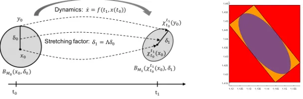
Figure 1: (Left) Visualization of one step of the Lagrangian Reachtube (LRT). The dashed arrows reflect the solution flowχof Eq. (1)(left). In this figure,δ0=ηξ0 andδ1=ηξ1. (Right)
Brusselator snapshot of the wrapping deficiency of Line 3 in Algorithm1.
an improved Lohner’s QR method [21,24] to account for the infamous wrapping effect, which is intrinsically connected to interval arithmetic [27]. For ease of presentation, we discuss our approach in the context of the Euler method, the simplest integration scheme available. Our prototype, however, supports also higher-order Runge-Kutta schemes.
This paper presents work in progress. The performance of our current implementation is still below that of one of our previous LRT tools on the benchmarks in [11, 12]. The reasons for the lower performance and various ways of improving it are discussed in Section5.
Notation. We denote by I the identity matrix in Rn×n, and by ∂x the partial derivative with respect to variablex. We denote byk · k2theEuclidean norm, and byk · k∞the maximum
norm. A similar notation is used for the induced operator norms. Following standard notation, the symbol0 stands for positive definiteness. For a given square matrixM 0, letBM(x, δ) be the closed ball with centerxand radiusδ >0 with respect to the metrickxkM :=
√
xTM x. The notation [x] is used for a box inRn, i.e., a product of compact intervals. We denote by mid([x]) and rad([x]) the midpoint and the radius of [x], respectively. We call ann×nmatrix [F] an interval matrix, if for all 1≤i, j≤n, the entries [F](i, j) of [F] are intervals.
2
Preliminaries
We study a system of nonlinear ODEs in unknown x∈Rn, as given in Eq. 1(left), with the corresponding system of variational equations in unknown ξ∈Rn, as given in Eq. 1(right), where the fieldf:Rn→
Rn is assumed to be a sufficiently smooth, time-invariant function (at least twice continuously differentiable):
∂tx=f(x), x0=x(t0) and ∂tξ= (∂xf)(x)·ξ, ξ0=ξ(t0). (1)
Since time dependence can be incorporated by adding the auxiliary variable ∂tx0 = 1 to the
system, our discussion naturally extends to time-varying systems of the form∂tx=f(t, x). The approach presented in this paper is based on our recent work on Lagrangian reachability (LRT), where the main idea is to use the Variational Eq. (1)(right), for obtaining a tight over-approximation [11,12]. More specifically, letχt1
t0 be the solution flow induced by Eq. (1)(left), i.e., χt1
t0(x0) = x(t1) when ∂tx=f(x) and x(t0) = x0. The gradient of the solution flow with respect to initial conditions, known as the sensitivity matrix [13,14], is defined by the function
x7→(∂xχtt10)(x) and satisfies, forξ0∈R
n and smallη∈
R, the relation:
χt1
t0(x0+ηξ0) =χ
t1
t0(x0) +η·(∂xχ
t1
t0)(x0)·ξ0+O(η
The above equation allows one to approximate χt1
t0(x0+ηξ0) using χ
t1
t0(x0) and (∂xχ
t1
t0)(x0), whenη is small. Moreover, the sensitivity matrix (∂xχtt10)(x0) can be related to the variational equations via (∂xχtt10)(x0)·ξ0=ξ(t1), provided thatξsatisfies∂tξ= (∂xf)(x)·ξ, withξ(t0) =ξ0, and that x obeys ∂tx = f(x) for x(t0) = x0 (see Chapter V, Theorem 3.1 in [16]). This
motivates us to consider the gradient of the flow matrix (called simply the gradient) F(t, x0)
that is given by the variational matrix equation ∂tF(t, x0) = (∂xf)(x(t))·F(t, x0). This is
because F(t1, x0)·ξ0 = ξ(t1), when ∂tξ = (∂xf)(x)·ξ for ξ(t0) = ξ0 and ∂tx = f(x) for
x(t0) =x0. Note that the two equations in (1) in particular imply thatF(t1, x0) = (∂xχtt10)(x0) holds.1
Next, we formally relate the over-approximation of (1) to its variational equations. To this end, we fix two matricesM0, M10 and consider as the initial regionBM0(x0, δ0), i.e., the ball in metric spaceM0centered atx0 with radiusδ0. Moreover, we chosey0 to be a point on the
surface ofBM0(x0, δ0) and setx 0
0=χ
t1
t0(x0) andy 0
0=χ
t1
t0(y0). Letδ1be the distance betweeny 0
0
andx00 in the metric space defined by matrixM1, as shown in Figure1(left).
The Cauchy Green stretching factor (SF) Λ measures the deformation of the ballBM0(x0, δ0) into the ballBM1(x
0
0, δ1), i.e., Λ =δ1/δ0. One can thus use the SF to bound the infinite set of
reachable states at timet1with the ball-overestimateBM1(χ
t1
t0(x0), δ1) in an appropriate metric
M10, which may differ fromM00. IfM1=M0 we refer to the computed SF asM0-SF or
M1-SF. Instead, ifM06=M1, we refer to the computed SF asM0,1-SF.
The correctness of the LRT approach is rooted in the following theorem.
Theorem 1(Thm. 1 in [12]). Lett0≤t1 be time points, andχtt10(x)be the solution att1 of the Cauchy problem (1), with initial condition(t0, x). LetM0, M1∈Rn×nwithM0, M10, and let
AT
0A0=M0,A1TA1=M1 be their respective decompositions. Let the ball in theM0-norm with
centerx0 and radius δ0,B=BM0(x0, δ0)⊆R
n, be a set of initial states for Eq. (1). Assume that there exists a compact enclosure[F]⊆Rn×n for the gradients F such that:
(∂xχtt10)(x)∈[F], ∀x∈ B. (3)
SupposeΛ>0 is an upper bound of the whole set ofM0,1 SFs [11], that is:
Λ≥
q
λmax (AT0)−1FTM1F A−01
=kA1F A−01k2, ∀F ∈[F], (4)
whereλmax represents the maximum eigenvalue. Then,
χt1
t0(x)∈BM1(χ
t1
t0(x0),Λ·δ0), (5) meaning that the reachable states at timet1 are contained in the ballBM1(χ
t1
t0(x0),Λ·δ0). In order to obtain a tight over-approximation, we wish to minimize Λ, the upper bound for theM0,1-SF given in Theorem1. Since finding the minimal value across allF ∈[F] is a difficult
task, we use the following heuristics. Given that the set [F] is represented by an interval matrix in our algorithm, we pick theM1 that minimizes theM1-SF with respect to mid ([F]), where
mid ([F]) is the value of F at the center of [F]. In [12], the following formula for such anM1,
conveniently denoted by ˆM1, has been obtained.
Theorem 2(Thm. 2 in [12]). Let (gradient)F ∈Rn×n have full rank andAˆ1,Mˆ1be such that
ˆ
A1(F) =V(F)−1 and Mˆ1(F) = ˆA1(F)TAˆ1(F), (6)
1Proof sketch:∂t(∂xχt
t0)(x) =∂x(∂tχ
t
t0)(x) =∂x(f(χ
t
t0))(x) = (∂xf)(χ
t
t0(x))·(∂xχ
Algorithm 1Lagrangian Reachability Algorithm [11,12].
Require: RealsCM, η >0, horizonT >0, maximal steph >0, timet0≥0, setBM0(x0, δ0)
1: setδ←δ0, δx←0, b←0, [F0]← {I}
2: while t0< T do
3: computeover-approximation [X] ofBM0(x0, δ0) in Cartesian coordinates
4: sett1←t0+ 2h
5: repeat
6: sett1←t0+12(t1−t0)
7: computeover-approximation [F1∗] of ∂xχtt10
([X]) 8: untilλ < η, whereλestimatesk[F∗
1]−[F0]k2
9: computetighter over-approximation [F1] of ∂xχtt10
([X]) for finalt1
10: computeΛ0as a bound of theM0-SF
11: compute optimal metric ˆM1(F) = ˆA1(F)TAˆ1(F) for F = mid ([F1]) (Thm. 2) and Λ1
as a bound of theM1-SF
12: if Λ0> CM ·Λ1 then
13: setΛ to a bound of theM0,1-SF (Thm.1)
14: setM1←Mˆ1, b←1, [F0]← {I}
15: else
16: setM1←M0, Λ←Λ0, [F0]←[F1]
17: end if
18: computeover-approximation [x1] ofχtt10(x0) andsetx1←mid([x1]),δx1 ←rad ([x1])
19: setδx←δx+δx1
20: setδ1←Λ·δ+δx (this specifiesBM1(x1, δ1) in full)
21: if b= 1 then
22: setδ←δ1, δx←0, b←0 (only if the norm is changed)
23: end if
24: set(M0, x0, δ0, t0)←(M1, x1, δ1, t1) (prepare for next iteration)
25: end while
where matricesV(F)andAˆ1(F)−1 contain the normalized eigenvectors of F. Then:
min A1∈Rn×n A1is invertible
Λ(A1, F) = Λ( ˆA1, F),
where the M1-SF is given by Λ(A1, F) =
q
λmax (AT1)−1FTM1F A−11
= A1F A−11
2. In
other words, the symmetric positive-definite matrixMˆ1= ˆAT1Aˆ1 minimizes theM1-SF.
3
Lagrangian Reachability Algorithm
Algorithm1summarizes the overall approach. Following [11,12], the choice of the current step sizet1−t0is adaptive and based on infinitesimal strain theory (IST). Specifically, the time-step
By invoking low-order schemes, we aim to improve the scalability of [11,12]. Previously, we appealed to the CAPD verification tool [7, 29,30], which utilizes high-order Taylor numerical schemes. To simplify the presentation, we next discuss only the Euler’s method. The wrapping effect is addressed by an improved version of the Lohner’s QR method [21, 24] and a careful choice of the next norm during the computation of the SF.
Computation of [X] in Algorithm1. The dynamical system specified by Eq. (1) is defined with respect to Cartesian coordinates (CC). In contrast, the over-approximation of the reachable statesBM0(x0, δ0) from the previous ball BMi(xi, δi) in one integration step is given in norm
M0. To work in CC, we first estimate BM0(x0, δ0) by a rectangle [X], as shown in line 3 of Algorithm1and Figure1(right). To this end, we first compute a rectangle [XM0] enclosing the ballBM0(x0, δ0) in theA
−1
0 coordinate system, whereM0=AT0 ·A0. Afterwards, we transform
[XM0] to CC (the orange box) to finally obtain [X] (the enclosing red box of [11,12]). Computation of[F]in Algorithm1. Letφti+1
ti be the solution flow induced by the variational matrix equations, i.e.,φti+1
ti (Fi, xi) =Fi+1when∂tF = (∂xf)(x)·F,F(ti) =Fi andx(ti) =xi. Given an interval matrix [Fi]⊆Rn×n, our goal is to compute the interval matrix [Fi+1] such
that φti+1
ti ([Fi],[Xi])⊆[Fi+1]. Due to the linearity of the variational equations, it holds that
φti+1
ti ([Fi],[Xi])⊆φ t0+hi
t0 (I,[Xi])·[Fi] withhi :=ti+1−ti [30]. This breaks down to finding an enclosure [Ji+1] such that φtt00+hi(I,[Xi])⊆[Ji+1]. Using the first order enclosure method [24], we compute rough enclosures [ ˜Xi] and [ ˜Ji] that satisfy:
h
[Xi] + [0, hi]·f([ ˜Xi])
i
⊆[ ˜Xi] withχ ti+1
ti ([Xi])⊆[ ˜Xi],
h
I+ [0, hi]·∂xf([ ˜Xi])·[ ˜Ji]
i
⊆[ ˜Ji] withφtt00+hi(I,[Xi])⊆[ ˜Ji].
As proposed in [30], we compute [ ˜Ji] by setting each element of the matrix to the interval [±max(el[0,hi])] and refine this enclosure by using the variational matrix equations related
to (1), where l denotes the logarithmic Euclidean norm of ∂xf([ ˜Xi]). Afterwards, the tight enclosure [Ji+1] is obtained by exploiting the relation:
[Ji+1]⊆I+hi∂xf([Xi])·I+
h2
i 2 ∂t
(∂xf)(x(t))·F(t, x)
[ ˜Xi], I
·[ ˜Ji]
| {z }
local truncation error
,
which underlies Euler’s method. By recalling that∂tF(t, x0) = (∂xf)(x(t))·F(t, x0), it holds
thatF(t+hi, x0) =F(hi, x(t))·F(t, x0), as has been observed in [30]. Hence:
[Fi+1] = [Ji+1]·[Fi]. (7) To allow for tight estimation, we do not evaluate the right-hand side of (7) using interval arithmetics. Instead, we pick a point matrix ˆFi∈[F], set [∆Fi] := [Fi]−Fˆi and write (7) as:
[∆Fi+1] = [Ji+1]·[∆Fi] + [∆Zi+1] (8)
where we set:
[Zi+1] = [Ji+1]·Fˆi−Fˆi+1, Fˆi+1= mid([Zi+1]), [∆Zi+1] = [Zi+1]−Fˆi+1.
To combat the wrapping effect, we use the Lohner’s QR factorization method, where in each step a new basisQi for [∆Fi] is chosen such that [∆Fi] =Qi·[∆FiQi] and that:
[∆FQi+1
i+1 ] = [Q
−1
i+1][Ji+1][Qi]
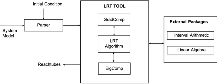
Figure 2: Overall architecture of our new stand-alone LRT tool. GradComp stands for Gradient Computation, and EigComp stands for Eigenvalue Computation.
At the first step, we set Q0 := I and ˆF0 = mid([F0]), thus ensuring [∆F0Q0] = [∆F0] =
0. In each step thereafter, the new coordinate system Qi+1 is chosen starting with Ui+1 =
mid ([Ji+1][Qi]). Following [24], the columns of Ui+1 are rearranged by a permutation matrix
Pi+1 such that the first column of ˜Ui+1(= Ui+1·Pi+1) corresponds to the longest edge of
Ui+1·[∆F
Qi
i ], the second column to the second longest, and so on. To obtain the new coordinate systemQi+1 we set it to the orthogonal matrix of the QR-factorization of ˜Ui+1. For a more
detailed discussion of the steps discussed above, please refer to [24] and [30].
Putting everything together. We are now in a position to explain Algorithm 1 in detail. More specifically, [xi+1] in line18is computed by applying Runge-Kutta of second order (RK2)
tof; instead, [F∗
1] in line7is computed by applying RK2 to the variational matrix equations,
without taking the local truncation error into account. This is faster than using Lohner’s method. Moreover, the absence of a rigorous bound is not critical because [F∗
1] is only used
to set the next timestep. Instead, [F1] in line 9 is obtained by applying Euler’s and Lohner’s
method to the variational matrix equations. Since [F1] is stored as an interval matrix, the
estimation of Λ0,Λ1 and Λ as the bounds for the M0-, M1- and M0,1-SF in the lines 10, 11
and14, respectively, amounts to the estimation of the largest eigenvalue; see also Theorem 1. To this end, we rely on the interval matrix algorithms of IBEX [2] and Eigen [1].
4
Tool Architecture
The LRT tool implements Algorithm 1 which is based on the fundamental research we pre-sented in [11, 12]. We ensure soundness of LRT by performing all computations in interval arithmetic [23], where a real-valued variable x is represented as an interval [x,x¯] such that
x≥xandx≤x¯. The architecture of the stand-alone LRT is illustrated in Figure2. Below we discuss each of its major components, which gives a complementary view of Algorithm1:
• Parser: The system dynamics and the initial condition are defined in two separate text files. Currently, we are using IBEX’s built-in functionality to parse the systems dynamics, and we implemented our own parser for the initial conditions.
∀x∈BM0(x0, δ0) it holds that (∂xχ
t1
t0)(x)∈[F1]
• Eigenvalue computation for [F1]: Given [F1], the next step of LRT is to compute
the maximum eigenvalue of the Cauchy-Green (CG) interval matrix CG = [F1]T·[F1],
which is a symmetric positive-definite interval matrix (tensor).2 To compute an upper
bound of the maximal eigenvalue of all symmetric matrices in some interval bounds, we implemented several algorithms from [17,26,25] and use the tightest result available.
• External Packages: For interval arithmetic and linear algebra operations, we use IBEX [2] C++library and Eigen [1] C++library, respectively.
5
Conclusion
The main motivation of our current work was to scale up (C)LRT to high-dimensional systems, for example, deep neural networks and the deep neural regulatory networks we have introduced in [20]. To this end, we considered the use of lower-order integration schemes, such as the advanced Runge-Kutta methods recently presented in [3], for the numerical computation of the (interval) sensitivity matrix [F]. The main reason behind this consideration is that computing the truncation order for high-dimensional systems is computationally prohibitive [3].
Other tools such as CAPD [7], which we used in [11, 12], also employ a variant of the C1-Lohner method to integrate the variational matrix equations of a given set of ODEs for obtaining [F]. CAPD, however, uses higher-order integration schemes based on the Taylor expansion, whereas we desire to keep the order low. Moreover, CAPD only uses the C1-Lohner method to combat the wrapping effect, while we combine it with a change of norm.
We conducted a preliminary evaluation of our stand-alone LRT tool on the benchmark mod-els from [11, 12]. We were able to recover the tight over-approximation of the 2-dimensional Brusselator, the 2-dimensional Mitchell-Schaeffer cardiac-cell model, and the 12-dimensional Polynomial System. The other models from [12], however, led to blowups in the over-approximation. CAPD [7], CORA [5] and Flow* [10] also seem to suffer from similar blowups if restricted to low-order schemes (or Taylor models). Hence, we will need to increase this order. We will also explore three ways of improving performance. First, we will seek to reduce the wrapping deficiency of line3 in Algorithm 1. This can be achieved by working in the Mi norm with both [Fi] andBMi(xi, δi), or by working in the Cartesian norm and employing a QR decomposition to support the use of the orange box shown in Figure1(right), instead of the red box. Second, we wish to obtain a better Cauchy Green SF. As per Theorem2, the tightness of the SF depends on the choice of metric Mi, which in turn depends on the eigenvalues of the particular Fi chosen out of [Fi]. Since theFi’s can significantly differ, we would like to explore genetic- or gradient-based techniques for their optimal choice. Third, we will improve the efficiency of the stand-alone LRT tool by tailoring it to specific classes of ODEs, in particular the ones corresponding to deep neural regulatory networks [20].
Acknowledgements. Sophie Gruenbacher is funded by FWF project W1255-N23. Max
Tschaikowski is supported by a Lise Meitner Fellowship funded by the Austrian Science Fund (FWF) under grant number M-2393-N32 (COCO).
2In fact we compute maximum eigenvalue of the CG matrix with the norm change: (AT
0) −1[FT
References
[1] Eigen Linear Algebra Library. http://eigen.tuxfamily.org. Copyright: Mozilla Public License Version 2.0.
[2] IBEX Interval Library. http://ibex-lib.org. Copyright: GNU Lesser General Public License. [3] J. Alexandre dit Sandretto and A. Chapoutot. Validated explicit and implicit Runge-Kutta
meth-ods. Reliable Computing (Electronic Edition), 22, July 2016.
[4] M. Althoff. Reachability analysis of nonlinear systems using conservative polynomialization and non-convex sets. InInternational Conference on Hybrid Systems: Computation and Control, pages 173–182, 2013.
[5] M. Althoff. An introduction to CORA 2015. InProc. of the Workshop on Applied Verification for Continuous and Hybrid Systems, 2015.
[6] M. Althoff, D. Grebenyuk, and N. Kochdumper. Implementation of Taylor models in CORA 2018. In Proc. of the 5th International Workshop on Applied Verification for Continuous and Hybrid Systems, pages 145–173, 2018.
[7] M. Capi´nski, J. Cyranka, Z. Galias, T. Kapela, M. Mrozek, P. Pilarczyk, D. Wilczak, P. Zgliczy´nski, and M. Zelawski. CAPD - computer assisted proofs in dynamics, a package for rigorous numerics, http://capd.ii.edu.pl/. Technical report, Jagiellonian University, Krak´ow, 2016.
[8] L. Cardelli, M. Tribastone, M. Tschaikowski, and A. Vandin. Maximal aggregation of polynomial dynamical systems.Proceedings of the National Academy of Sciences, 114(38):10029 – 10034, 2017. [9] L. Cardelli, M. Tribastone, M. Tschaikowski, and A. Vandin. Guaranteed error bounds on approx-imate model abstractions through reachability analysis. InInternational Conference on Quanti-tative Evaluation of SysTems, pages 104–121, 2018.
[10] X. Chen, E. ´Abrah´am, and S. Sankaranarayanan. Flow*: An analyzer for non-linear hybrid systems. InCAV’13, the 25th International Conference on Computer Aided Verification, pages 258–263, Saint Petersburg, Russia, July 2013. Springer.
[11] J. Cyranka, M. A. Islam, G. Byrne, P. Jones, S. A. Smolka, and R. Grosu. Lagrangian reachabililty. In R. Majumdar and V. Kunˇcak, editors,CAV’17, the 29th International Conference on Computer-Aided Verification, pages 379–400, Heidelberg, Germany, July 2017. Springer.
[12] J. Cyranka, M. A. Islam, S. A. Smolka, S. Gao, and R. Grosu. Tight Continuous-Time Reachtubes for Lagrangian Reachability. InCDC’18, the 57th IEEE Conference on Decision and Control, pages 6854–6861, Miami Beach, FL, USA, December 2018. IEEE.
[13] A. Donz´e. Breach, a toolbox for verification and parameter synthesis of hybrid systems. InCAV’10, the 22nd International Conference on Computer Aided Verification, pages 167–170, Edinburgh, UK, July 2010. Springer.
[14] A. Donz´e and O. Maler. Systematic simulation using sensitivity analysis. InInternational Work-shop on Hybrid Systems: Computation and Control, pages 174–189. Springer, 2007.
[15] G. Frehse, C. Le Guernic, A. Donz´e, S. Cotton, R. Ray, O. Lebeltel, R. Ripado, A. Girard, T. Dang, and O. Maler. Spaceex: Scalable verification of hybrid systems. InCAV’11, the 23rd International Conference on Computer Aided Verification, pages 379–395, Snowbird, Utah, USA, July 2011. Springer.
[16] P. Hartman. Ordinary Differential Equations. SIAM, 1982.
[17] M. Hladik, D. Daney, and E. Tsigaridas. Bounds on real eigenvalues and singular values of interval matrices.SIAM Journal on Matrix Analysis and Applications, 31(4):2116–2129, 2010.
[18] M. A. Islam, A. Murthy, A. Girard, S. A. Smolka, and R. Grosu. Compositionality results for cardiac cell dynamics. InInternational Conference on Hybrid Systems: Computation and Control, pages 243–252, 2014.
[20] M. Lechner, R. Hasani, M. Zimmer, T. Henzinger, and R. Grosu. Designing worm-inspired neural networks for interpretable robotic control. InICRA’19, the 2019 IEEE International Conference on Robotics and Automation, Montreal, Canada, May 2019. IEEE.
[21] R. Lohner.Computation of guaranteed enclosures for the solutions of ordinary initial and boundary value problems, chapter Computational Ordinary Differential Equations. Clarendon Press, Oxford, 1992.
[22] M. Martel and O. Bouissou. GRKLib: a Guaranteed Runge Kutta Library. In2006 12th GAMM-IMACS International Symposium on Scientific Computing, Computer Arithmetic and Validated Numerics (SCAN), volume 00, page 8, 2006.
[23] R. E. Moore. Interval analysis. Series in automatic computation. Englewood Cliff: NJ Prentice-Hall, 1966.
[24] N. Nedialkov, K. Jackson, and G. Corliss. Validated solutions of initial value problems for ordinary differential equations. Applied Mathematics and Computation, 105(1):21 – 68, 1999.
[25] J. Rohn. Bounds on eigenvalues of interval matrices. ZAMMZ.Angew.Math.Mech., 78:1049–1050, 1998.
[26] S. M. Rump. Computational error bounds for multiple or nearly multiple eigenvalues. Linear Algebra and its Applications, 324(1):209 – 226, 2001. Linear Algebra in Self-Validating Methods. [27] J. K. Scott and P. I. Barton. Bounds on the reachable sets of nonlinear control systems.Automatica,
49(1):93 – 100, 2013.
[28] M. Tschaikowski and M. Tribastone. Approximate reduction of heterogenous nonlinear models with differential hulls.IEEE Trans. Automat. Contr., 61(4):1099–1104, 2016.
[29] D. Wilczak and P. Zgliczy´nski. Cr-Lohner algorithm. Schedae Informaticae, 2011(Volume 20), 2012.