Regional variability of acidification in the Arctic: a sea of contrasts

www.biogeosciences.net/11/293/2014/ doi:10.5194/bg-11-293-2014

© Author(s) 2014. CC Attribution 3.0 License.

Biogeosciences

Regional variability of acidification in the Arctic: a sea of contrasts

E. E. Popova, A. Yool, Y. Aksenov, A. C. Coward, and T. R. Anderson

National Oceanography Centre, University of Southampton Waterfront Campus, European Way, Southampton SO14 3ZH, UK

Correspondence to: E. E. Popova (ekp@noc.ac.uk)

Received: 29 January 2013 – Published in Biogeosciences Discuss.: 18 February 2013 Revised: 6 December 2013 – Accepted: 9 December 2013 – Published: 23 January 2014

Abstract. The Arctic Ocean is a region that is particularly

vulnerable to the impact of ocean acidification driven by rising atmospheric CO2, with potentially negative

conse-quences for calcifying organisms such as coccolithophorids and foraminiferans. In this study, we use an ocean-only gen-eral circulation model, with embedded biogeochemistry and a comprehensive description of the ocean carbon cycle, to study the response of pH and saturation states of calcite and aragonite to rising atmosphericpCO2and changing

cli-mate in the Arctic Ocean. Particular attention is paid to the strong regional variability within the Arctic, and, for com-parison, simulation results are contrasted with those for the global ocean. Simulations were run to year 2099 using the RCP8.5 (an Intergovernmental Panel on Climate Change (IPCC) Fifth Assessment Report (AR5) scenario with the highest concentrations of atmospheric CO2). The separate

impacts of the direct increase in atmospheric CO2and

indi-rect effects via impact of climate change (changing tempera-ture, stratification, primary production and freshwater fluxes) were examined by undertaking two simulations, one with the full system and the other in which atmospheric CO2was

pre-vented from increasing beyond its preindustrial level (year 1860). Results indicate that the impact of climate change, and spatial heterogeneity thereof, plays a strong role in the de-clines in pH and carbonate saturation () seen in the Arctic. The central Arctic, Canadian Arctic Archipelago and Baf-fin Bay show greatest rates of acidification anddecline as a result of melting sea ice. In contrast, areas affected by At-lantic inflow including the Greenland Sea and outer shelves of the Barents, Kara and Laptev seas, had minimal decreases in pH andbecause diminishing ice cover led to greater ver-tical mixing and primary production. As a consequence, the projected onset of undersaturation in respect to aragonite is highly variable regionally within the Arctic, occurring during the decade of 2000–2010 in the Siberian shelves and

Cana-dian Arctic Archipelago, but as late as the 2080s in the Bar-ents and Norwegian seas. We conclude that, for future pro-jections of acidification and carbonate saturation state in the Arctic, regional variability is significant and needs to be ade-quately resolved, with particular emphasis on reliable projec-tions of the rates of retreat of the sea ice, which are a major source of uncertainty.

1 Introduction

The concentration of CO2has been steadily rising in the

at-mosphere as a result of the burning of fossil fuels, cement manufacture and land-use changes (Friedlingstein et al., 2010). Further increases are expected on the basis of current emission rates, e.g. to 450–650 ppm by the mid 21st century (Peters et al., 2012). The ocean acts as a sink for this atmo-spheric carbon, with uptake estimated at 120–140 Pg C since preindustrial times (Sabine et al., 2004; Khatiwala et al., 2009). The invasion of CO2 into the ocean has two

impor-tant consequences for seawater chemistry, namely that both pH and carbonate saturation state () decrease. The ocean biota, and especially calcifying organisms such as coccol-ithophores, foraminiferans and pteropods, are particularly vulnerable to these changes (Fabry et al., 2008; Gangstøet al., 2011).

In addition to the direct impact of CO2invading the ocean,

pH and saturation state are influenced by other aspects of changing climate, including temperature increase, changes in upper ocean mixing (including associated changes in net pri-mary production), retreating sea ice and increasing freshwa-ter input. A number of studies have examined the relative im-portance of the direct impact of invading CO2and these other

the most important of the climate change factors. It has rel-atively little effect on pH because, although increasing tem-perature causes pH to decrease, it also buffers dissolved in-organic carbon (DIC) increase (and associated pH decrease) through the reduction in CO2solubility. In contrast,

carbon-ate saturation stcarbon-ate, which is relatively insensitive to the di-rect effect of temperature, declines significantly because of increasing DIC in the ocean, despite the buffering effect of temperature. The implication is that future projections of sur-face ocean acidification (pH) in the global ocean need only consider the direct effect of CO2invading the ocean, whereas

the temperature effect is more relevant regarding carbonate saturation state.

The Arctic is an area that is particularly sensitive to chang-ing climate (Walsh et al., 2011) as a result of so-called polar amplification (Moritz et al., 2002). Observations have shown that a number of areas in the Arctic Ocean (AO) are already undersaturated with respect to aragonite (e.g. the Canada Basin: Yamamoto-Kawai et al., 2009; freshwater-influenced shelves: Chierici and Fransson, 2009; the Chukchi, Beaufort and eastern East Siberian seas: Bates et al., 2011). A num-ber of modelling and observational studies have indicated that the Arctic Ocean, with its low temperatures, substan-tial freshwater input and fast retreating sea ice, is a region where the impact of ocean acidification is likely to mani-fest itself first (McNeil and Matear, 2007; Yamamoto-Kawai et al., 2009; Yamamoto et al., 2012, Steinacher et al., 2009; Bates et al., 2011). Future declines in pH andhave been shown to closely track changes in atmospheric CO2. The

equilibration between oceanic and atmospheric CO2follows

the well-established carbonate chemistry of sea water, with only a relatively minor impact by the changing ocean physics in nearly all ocean regions except for the Arctic Ocean (e.g. Yamamoto et al., 2012; McNeil and Matear, 2007). The fast retreat of sea ice leads to the exposure of previously under-saturated (with respect to CO2) areas to the atmosphere,

ac-celerating its absorption by the ocean. Other potential im-pacts include changes in stratification with consequences for nutrient supply and primary productivity (e.g. Popova et al., 2010), and the effect of freshwater input (Chierici and Frans-son, 2009).

Various climate-related impacts on ocean acidification have been included in modelling studies, and have indicated that the Arctic Ocean will become undersaturated with re-spect to aragonite by the 2040s (e.g. Steinacher et al., 2009; Yamamoto et al., 2012). These studies generally assessed the impact of acidification in the Arctic on the basis of basin-averaged or zonal characteristics. The Arctic Ocean is, how-ever, an area with large spatial gradients in physical and bio-logical properties (e.g. Carmack et al., 2006; Popova et al., 2010);even more importantly, it is an area where climate change factors are expected to have strong regional varia-tions. In this paper we focus on regional aspects of Arc-tic Ocean acidification, with two main aims. First, using a global ocean general circulation model (OGCM), we

in-vestigate the direct (invasion of CO2) and indirect

(climate-related) effects of increasing atmospheric CO2 (changes in

temperature, stratification, sea ice cover and freshwater in-put) on pH and saturation state in the Arctic Ocean, under-taking an intercomparison with the rest of the global ocean. The OGCM includes a full representation of the carbon cycle and is forced by the atmospheric CO2concentration through

the period 1860–2099 from an Earth system model run un-der the RCP8.5 scenario (Jones et al., 2011). This run is de-scribed and analysed in detail for the global ocean by Yool et al. (2013b). The second aim is to study the heterogeneity of acidification and carbonate saturation state in the Arctic as projected by the model, and to relate it to the variability in underlying factors. The direct and indirect effects are distin-guished by comparing two parallel simulations of the model. The first run is that described above, where the ocean carbon system experiences both increasing atmospheric CO2and the

resulting climate impacts on ocean physics and biology. The second simulation separates CO2and climate by holding

at-mospheric CO2constant at the year 1860 value while

contin-uing to allow climate change.

Recent modelling studies analysing the output of multi-model experiments have found significant inter-multi-model dif-ferences in the Arctic Ocean (e.g. Steinacher et al., 2010; Popova et al., 2012, Steiner et al., 2014). Thus care should be taken when interpreting the results presented in this study in view of the uncertainty in the projected changes. Although this study presents a detailed analysis of underlying physi-cal and biogeochemiphysi-cal mechanisms, it is based on a single model and is therefore less robust than those based on multi-model projections, e.g. Tebaldi and Knutti (2007).

2 Method

cycles, atmospheric chemistry and aerosols (Collins et al., 2011). The HadGEM2-ES simulation used here, identifier AJKKH, was performed as part of the UKMO’s input (Jones et al., 2011) to the Coupled Model Intercomparison Project 5 (CMIP5) and Assessment Report 5 (AR5) of the Intergovern-mental Panel on Climate Change (IPCC). The frequency of output fields is monthly for precipitation (rain, snow, runoff), daily for radiation (downwelling short- and long-wave) and 6 hourly for the turbulent variables (air temperature, humid-ity and wind velocities). Biogeochemical model is forced by the atmospheric CO2 concentrations of the HadGEM2-ES

run under the RCP8.5 scenario (Yool et al., 2013b). A caveat of such an approach is that the atmospheric CO2we use for

the forcing was affected by the HadGEM2-ES ocean model, which is not consistent with the ocean physics and biogeo-chemistry of the model used in this study.

In order to separate the impacts of rising atmospheric CO2

from those of changing climate (imposed on the ocean model through the boundary conditions of physical variables), we perform a second simulation in which atmospheric CO2 is

held constant at the value for year 1860 while continuing to allow climate change.

Biogeochemistry in NEMO is represented by the plank-ton ecosystem model MEDUSA (Model of Ecosystem Dy-namics, carbon Utilisation, Sequestration and Acidification; Yool et al., 2011, 2013a). This is a size-based, intermediate-complexity model that divides the plankton community into “small” and “large” portions and which resolves the ele-mental cycles of nitrogen, silicon and iron. The small por-tion of the ecosystem is intended to represent the micro-bial loop of picophytoplankton and microzooplankton, while the large portion covers microphytoplankton (specifically di-atoms) and mesozooplankton. The intention of MEDUSA is to separately represent small, fast-growing phytoplankton that are kept in check by similarly fast-growing protistan zooplankton and large, slower-growing phytoplankton that are able to temporarily escape the control of slower-growing metazoan zooplankton. The non-living particulate detritus pool is similarly split between small, slow-sinking particles that are simulated explicitly and large, fast-sinking particles that are represented only implicitly. See Yool et al. (2013a) for a full description of the model. The riverine input of all biogeochemical state variables is prescribed through a no-flux boundary condition similar to that of temperature, where river water implicitly has the same concentrations as the sea-water it mixes into. Note thatis calculated as a function of salinity, which is zero in the riverine water (Yool et al., 2013b). Concentration of all biogeochemical state variables in the rain, snow and ice melt water is assumed to be zero. The model does not account for the glacier melt.

Model performance with respect to ecosystem dynamics of the present-day Arctic Ocean was assessed by Popova et al. (2010, 2012, 2013) and globally by Yool et al. (2011). Model performance with respect to the global ocean carbon cycle is described in Yool et al. (2013a, b). For the Arctic

Ocean we note good agreement of modelled values of surface saturation with respect to calcite (c), and aragonite (a)

with values reported by Jutterström and Anderson (2005) for the central Arctic Ocean (1.9–2.7 forcand 1.1–1.8 for

ameasured during 1990s). Over the shelves of the western

Arctic Ocean and Baffin Bay the modelled values are in the same range as observations reported by Chierici and Frans-son (2009) (8.0–8.2 for pHSWS, where SWS denotes sea

wa-ter scale units; 1.8–3.0 forc1.8–2.0 for fora); however

we note that the model underestimates high values ofcand

ain the Chukchi Sea (4 and 2.5 as reported by Chierici and

Fransson, 2009, and Bates et al., 2012) by about 1 unit. In Sect. 3.3 we evaluate the sensitivity of our main results to uncertainties in the parameterisations of the main factors that control them with a focus on the rate of sea ice de-cline and ocean mixing. Variation in the rate of ice dede-cline is achieved by varying (i) albedo of snow/ice surface, (ii) bulk sea ice salinity, and (iii) partitioning between basal and lat-eral oceanic heat fluxes towards sea ice. The albedo experi-ments introduce two sensitivity cases to the control simula-tions, the faster ice melting and the slower ice melting. In the former case, following Shine and Henderson-Sellers (1985) albedo formulation, we decrease the albedo for the snow/ice classes to 0.60 for frozen bare ice, to 0.40 for melting ice, to 0.75 for dry and 0.52 for thick melting snow (the control run uses values of 0.72, 0.50, 0.80 and 0.65 respectively). To slow down sea ice melting, the above parameters are taken as 0.72, 0.58, 0.87 and 0.70. The ranges of the albedo variations are designed to emulate changes in the surface properties of the snow and ice cover.

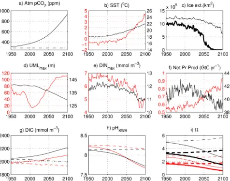
Fig. 1. Time evolution of modelled characteristics for the global

ocean (black line and font) and the Arctic Ocean (treated as north of 66◦N, red line and font): (a) atmospheric CO2 (ppm) from

the forcing Earth system model; (b) sea surface temperature (◦C);

(c) extent of the Northern Hemisphere sea ice (km2) for September (thick line) and March (thin line); (d) maximum depth of the up-per mixed layer UML, (m); (e) annual maximum surface dissolved inorganic nitrogen (DIN, mmol m−3); (f) water-column-integrated net primary production (g C yr−1); (g) surface DIC (mmol m−3);

(h) pHSWS; (i)canda. Annual mean characteristics are given

for all properties unless otherwise specified. For (g–i) dashed lines refer to the “climate-effect” run (no CO2increase); for (i) thin line

refers toc, thick line refers toa.

3 Results

3.1 Regional aspects of Arctic Ocean acidification

Under the RCP8.5 scenario, atmospheric CO2 in the

HadGEM2-ES model (used here as forcing) reaches 950 ppm by the end of the century. Projected by NEMO, globally averaged SST (sea surface temperature) rises from 18 to 22◦C during the same period (Fig. 1a, b). This in-crease is more pronounced in the Arctic Ocean (defined here as north of 66◦N) due to polar amplification (Moritz et al., 2002), with SST changing from−1 to 4.5◦C (Fig. 1b). The associated decline of sea ice leads to virtually ice-free condi-tions in summer in the Arctic Ocean from the 2060s onwards (Fig. 1c).

Ice retreat is the factor that most strongly influences the spatial distribution of the projected declines of pHSWSand

in the Arctic Ocean (e.g. McNeil and Matear, 2007). This is a result of increasing ocean uptake of CO2, freshening of the

surface layers by melt of the perennial ice and the deepening of winter mixing. Modelled annual mean sea ice concentra-tion for years 2000 and 2099 is shown in Fig. 2a and b. Sea-sonally ice-free conditions in the Arctic Ocean occur during the decade of the 2060s. By the end of the 21st century, the

Fig. 2. Arctic Ocean annual mean ice concentration for year

2000 (a), 2099 (b), difference between year 2099 and 2000 (c). The red line on this and subsequent Arctic plots shows 500 m bathymet-ric contour.

Fig. 3. Arctic Ocean surface salinity (a, b), maximum upper mixed

layer depth (UML) (c, d) in m, net primary production (a–c) in g C m−2yr−1. The first column shows values for year 2099; the sec-ond column shows deviation between year 2099 and year 2000.

central Arctic Ocean becomes nearly ice-free on an annual basis and winter ice occurs only on the Siberian and Cana-dian shelves, including Baffin Bay (Fig. 2b). The retreat of the ice brings substantial changes to projected surface salin-ity (Fig. 3a, b), with a strong decline over the shelves of the western Arctic Ocean and in Baffin Bay of up to 3 driven by the accumulation of the melt water. The second major area of salinity decline is the Siberian shelves (up to 4 due to the increase in riverine input). In the areas which change from being permanently ice-covered to permanently ice-free (the central Arctic Ocean), surface salinity increases by about 3– 4. In addition, an increase in surface salinity occurs in areas of deepening winter mixing, mostly associated with Atlantic inflow (Fig. 3c, d).

of acidification, since it controls exchange with deeper lay-ers that have higher salinity, temperature, nutrients, and DIC. During the simulation, winter mixing deepens over the ma-jority of the Arctic Ocean (Fig. 3c, d), with the exception of the Norwegian and western Barents seas, where ocean warm-ing induces shallowwarm-ing of winter mixwarm-ing by more than 200 m. The greatest deepening of winter mixing occurs in areas of increased Atlantic inflow into the Arctic Ocean, namely the Greenland Sea and the outer shelves of the Barents, Kara and Laptev seas, where deep mixing by the end of the century penetrates to 200–300 m.

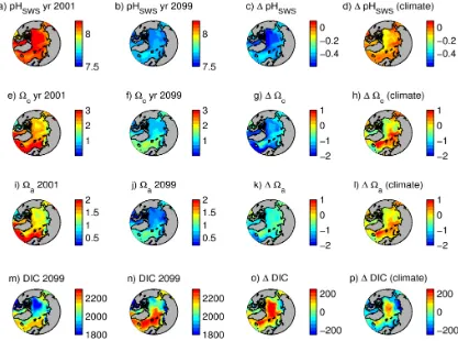
The areas experiencing the largest changes in ice regime (from permanent ice cover as it is today to a year-round ice-free zone by 2099) and substantial freshening show the largest decreases in pHSWS from 8.2 to 7.65 (central

Arc-tic Ocean, Canadian ArcArc-tic Archipelago and Baffin Bay, Fig. 4a, b),cfrom 2 to 1 (Fig. 4e, f) and a from 1.2

to 0.5 (Fig. 4i, j). The largest increase in DIC is also seen in the central AO (Fig. 4m, n) due to equilibration with the atmosphere following the loss of permanent ice cover. About half of this increase (100–110 out of 220 mmol m−3) happens as a result of the climate change impact driving retreat of the ice (Fig. 4o, p).

Now we aim to achieve more quantitative estimates of the role of various factors across the Arctic Ocean. This requires us to more formally define the boundaries of the Arctic do-mains where the relative importance of these factors is dif-ferent. pHSWSandare dependent on total alkalinity (Alk),

DIC, temperature (T) and salinity (S). Each of these vari-ables is affected by freshwater input and by advective and diffusive processes. Alk and DIC are also modified by the ocean biota (e.g. photosynthesis, respiration, calcification), while DIC is additionally affected by air–sea gas exchange. In this section we estimate which processes are most respon-sible for changes in pHSWS and over the period 2000–

2099, and how their relative contributions vary across the Arctic Ocean. The processes identified are air–sea gas ex-change, freshwater input, vertical mixing, advection, hori-zontal diffusion, biological process, and changes inT andS. Note that, in the case of changes inT andS, we consider their total impact on pHSWSandwithout separation between

ad-vection, diffusion and fluxes at the ocean–atmosphere bound-ary. We evaluate the contributions of each of these processes in the upper 100 m for every model grid point of the Arctic Ocean, following the approach of Yamamoto et al. (2012). However, unlike this study, here we obtain spatial distribu-tions of the factors in question, rather than total Arctic bud-gets.

The spatial distributions of the contributing factors (re-sults not shown) show strong regional variability that broadly forms four distinctive provinces, each manifesting qualita-tively different flux balances. The spatial extents of these provinces are shown in Fig. 5a. Specifically, we define the following provinces: (1) Siberian shelves (areas of less than 220 m depth in the Kara, Laptev, East Siberian and Chukchi

seas); (2) Atlantic inflow (areas where diffusivity makes a substantial contribution to the 100 m budget imposing de-cline ofain excess of 0.1); (3) Nordic minimum (area of

minimumachanges in the Arctic Ocean over the century,

defined as areas where these changes do not exceed 0.9); and (4) freshwater province (areas where freshwater fluxes play dominant role in theachanges, defined as areas not covered

by i–iii). Although some of the exact numerical definitions of the domain boundaries are somewhat subjective, we find these selection criteria to be most successful at delineating the qualitative differences across the AO.

Projected changes inabetween year 2000 and 2099 for

the Arctic Ocean (defined as north of 66◦N) and the four provinces defined above are shown in Fig. 5b. As described previously, Fig. 5b also breaks this total change down into contributions due to the process described above except for horizontal diffusion and those due to changes in T andS which were found to be negligible.

Decline ofaover the Siberian shelves occur slower than

in other provinces with the exception of Nordic minimum. However, by 2099 values of pHSWS andare lower than

those in the central Arctic Ocean since present-day pHSWS

andare already low in this area. Thus, by 2099 surface pHSWS is as low as 7.6, while typical valuescandaare

0.8 and 0.4 respectively. In these areas, the impact of air– sea gas exchange is relatively low due to high concentrations of DIC, while those of vertical diffusivity and freshwater from ice melt, which strongly reduceain other provinces,

are nearly negligible. The main factor reducinga in this

province is horizontal advection of riverine water, which is nearly compensated for by the biological pump (Fig. 5b).

The Atlantic inflow province is characterised by strong de-creases inadriven by vertical diffusivity, horizontal

advec-tion and air–sea gas exchange, with a relatively weak com-pensating effect of the biological pump (Fig. 5b). Although the rate of change ina over the century in this province is

the highest in the Arctic Ocean, this area is projected to re-main oversaturated by the end of the century in respect to aragonite due to its high present-day values (Fig 4m, n, o) influenced by the upstream North Atlantic.

The Nordic minimum province was identified on the ground of slowest changes in the a. All of these decline

over the 21st century and are clearly buffered by the physical changes (cf. Fig. 4 panels g and h, k and l, and o and p). We note that this province is also characterised by a substantial deepening of winter mixing (Fig. 3d). Analysis of the budget fluxes shows that, in spite of this deepening, vertical diffu-sivity does not play a major role in controllinga directly.

Instead, the low rate ofadecline is driven here by relatively

Fig. 4. Arctic Ocean pH_SWS(a–d),c(e–h),a(i–l), DIC (mmol m−3, m–n). The first and second columns shows values for year 2000

and 2099 respectively, the third column shows deviation between year 2099 and year 2000 for the full run, and the fourth column shows deviation between year 2099 and year 2000 for the for the climate change run.

As can be seen from Fig. 5a, the freshwater province occupies the central Arctic Ocean, the Canadian Arctic Archipelago, Baffin Bay and the Greenland Sea. These ar-eas experience the largest changes in the ice regime, from near-permanent ice cover today through to year-round ice-free conditions by 2099. Freshwater flux is the largest con-tributing factor in the decline of a within this province,

though this is largely counterbalanced by advective fluxes since the province also includes the main areas of AO out-flow. Gas exchange also plays substantial role in reducinga

following the loss of the permanent ice cover that previously prevented equilibration with the atmosphere. The province maintains its very stable stratification across the 21st century such that vertical diffusivity does not significantly contribute to the 100 m balance. A further notable feature is the com-pensating effect of the biological pump which increases with productivity over some of the province as it transitions across the 21st century to an ice-free state.

In summary, these results indicate climate change has pro-nounced, if regional, impacts onin the Arctic Ocean. Fac-tors such as freshwater input from melting of (previously) permanent ice cover, advection of riverine freshwater and

vertical diffusive fluxes vary strongly spatially and result in regionally variable impacts in the decline ofa. Although

not presented here, a similar budget analysis for pHSWS

shows similar variability across the main domain with an additional impact of temperature dependence (McNeil and Matear, 2007). In some regions of the Arctic Ocean, climate change increases the decline of pHSWSandby up to factor

of 2 relative to rising atmospheric CO2. Meanwhile, in other

areas it nearly cancels (buffers) changes induced by rising CO2. Thus, processes driven by climate change create strong

gradients in the rates of decline of pHSWS andacross the

basin.

3.2 Timing of the first occurrence of undersaturation conditions in the Arctic Ocean

Fig. 5. (a) Spatial extent of four provinces showing qualitatively

different balance of the main factors contributing to the a

de-cline over the 21st century and identified as Siberian shelves (dark blue), Atlantic inflow (light blue), Nordic minimum (green), fresh-water province (orange) – see text; (b) projected changes in the an-nual mean difference inafrom 2000 to 2099 in the top 100 m of

the Arctic Ocean (north of 66◦N, dark red bars) and four province shown in (a). The total change (1Om) is divided into contribution by air–sea gas exchange (Air–Sea), biology (Bio), freshwater fluxes (Fr.W), vertical diffusivity (V.Dif), and advection (Adv).

marine organisms such as shellfish that form the basis of regional fisheries, it is crucial to estimate the time of the onset of undersaturation. The year of first occurrence of monthly mean undersaturated surface waters with respect to calcite and aragonite under the RCP8.5 scenario is shown in Fig. 6a and b, while the same characteristic for shelf bot-tom waters is shown in Fig. 6c and d. With respect to arag-onite, undersaturation of both surface and bottom waters is already widespread at the Siberian shelves, Canadian Arc-tic Archipelago and part of the Beaufort Sea affected by the McKenzie River. The surface of the Beaufort Gyre becomes undersaturated before 2020, followed by widespread under-saturated conditions in the central Arctic before 2040. Areas affected by the Atlantic inflow become undersaturated last, during the 2080s.

In the case of calcite, undersaturation in the surface occurs 20–30 yr later than that of aragonite, and follows the same spatial progression (Fig. 6a, c). Siberian shelves become

un-Fig. 6. The first occurrence of a monthly mean undersaturated

sur-face waters in respect to calcite (a) and aragonite (b, years). The same for the shelf bottom waters at the depth of the deepest model vertical grid box (c, d).

dersaturated first, starting from the inner shelves of the Kara and Laptev seas and Canadian Arctic Archipelago, followed by the central Arctic Ocean. Areas affected by the Atlantic inflow (Greenland, Norwegian and Barents seas) do not show undersaturation within the 21st century. Shelf bottom water shows a similar timing of calcite undersaturation, except for the East Siberian Sea, where undersaturation at the bottom occurs nearly two decades earlier than at the surface.

The timing of the onset of undersaturated conditions pre-sented in this section is based on the first occurrence of a monthly mean undersaturated value. The season in which such conditions are likely to first occur depends on the ampli-tude and phase of the annual cycle. Our results find that, rel-ative to the projected change through the century, the annual amplitude ofais relatively low in the central AO

(approx-imately 0.1–0.2), though higher (approx(approx-imately 0.3–0.4) in areas affected by Pacific or Atlantic inflow. This amplitude remains nearly unchanged through the 21st century even in the face of large absolute change in a during this period.

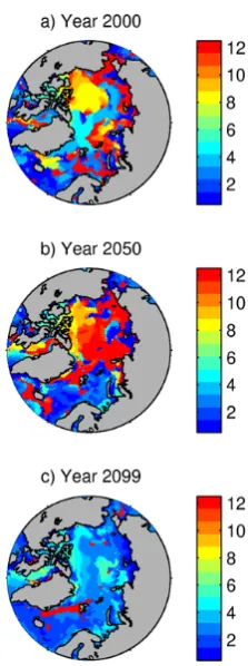
However, the phase of the annual cycle varies strongly, both in space across the basin and in time through the 21st century. Fig. 7 shows the timing of minimum annual values (month number) across the Arctic Ocean for years 2000, 2050 and 2099. As the Arctic Ocean progresses into an ice-free state towards the end of the century, the phase of the annual cycle ina becomes similar to that at mid-latitudes with a

Fig. 7. Number of the month (January = 1) in which minimum

annual values ofaoccur in year 2000 (a), 2050 (b) and 2099 (c).

minima across the AO occur throughout the year. The study of Steinacher et al. (2009) found that latitudinally averaged seasonality in the Arctic Ocean is generally out of phase with the seasonal signal in the rest of the northern hemisphere due to the impact of freshwater input from melting sea ice. Our results show a similar trend to that found by Steinacher et al. (2009) in the areas most affected by freshwater input from melting ice, but the opposite situation in areas of Pacific or Atlantic inflow. A transitional zone exists between these ar-eas which is influenced by strong temporal and/or regional differences in the depth of winter mixing. In summary, pro-jecting the season in which one might expect undersaturation conditions to first occur in the Arctic Ocean is a complex is-sue driven in part by future climate change but also by the underlying complexity in the spatial and temporal variability of the phase of theaannual cycle.

3.3 Sensitivity experiments

In this section we evaluate the sensitivity of our main re-sults to uncertainties in the parameterisations of the main fac-tors that control them. The high computational cost of global model runs (even at relatively modest resolution) permits us to focus only on the major physical processes that affect rates of acidification but which are known to be poorly constrained

in the climate models. Namely the rate of the decline of Arc-tic sea ice and oceanic verArc-tical mixing (e.g. Yamamoto et al., 2012, Popova et al., 2012). With this purpose in mind, we performed four additional sensitivity experiments: (1) faster ice decline; (2) slower ice decline; (3) lower mixing; and (4) higher mixing.

The numerical experiments were run for 100 yr, starting from the control run state corresponding to the year 2000. Both sets of sensitivity experiments (variation in the rates of ice decline and vertical mixing) lead to substantial modifi-cations to both Arctic Ocean physics and biogeochemistry. We focus our attention here on the sensitivity of the pro-jected first occurrence of the undersaturated – with respect to aragonite – surface waters (Fig. 6b), henceforth referred to as “undersaturation onset” for brevity.

The temporal evolution of Northern Hemisphere minimum ice extent (September) and Arctic-averageda for the

con-trol and numerical experiments are shown in Fig. 8a and b. In the ice decline simulations, the Arctic Ocean becomes sea-sonally ice-free approximately 15 yr earlier or later than in the control run. Values of Arctic-averageda are lower in

the simulations with faster ice decline or lower diffusivity (and marginally higher with slower ice decline or higher dif-fusivity), although the deviation between the control run and experiments does not exceed 0.05 (Fig. 8a, b) in the first half of the century and becomes negligible in the second half.

However, as Fig. 8c–f show, the regional variability of the differences in undersaturation onset between the control run and the sensitivity experiments is substantial. The area most sensitive to the change in the rate of ice decline is the Beau-fort Gyre, showing acceleration of the undersaturation onset by about 20 yr, especially at its periphery in the case of faster ice decline. In the case of slower ice decline, the centre of the gyre shows a delay in undersaturation onset of approxi-mately similar duration. The Beaufort Gyre manifests simi-larly high sensitivity in the experiments with variable vertical diffusivity (Fig. 8e,f). In the lower diffusivity run (Fig. 8e), undersaturation onset occurs about 10–20 yr earlier, with the maximum of the signal again at the periphery of the gyre. Meanwhile, in the higher diffusivity experiment (Fig. 8f), it occurs about 8–12 yr later with the maximum signal located instead in the centre of the gyre.

Fig. 8. Time evolution of the modelled characteristics for the Arctic Ocean (treated here as poleward of 66◦N): (a) extent of the Northern Hemisphere sea ice (September averaged, km2); (b)afor the control run (black); fast (red) and slow ice decline (blue); high (green) and

low (magenta) diffusivity experiments; (c–f): difference in the date (years) of the first occurrence of undersaturated conditions in respect to aragonite between the control run and the following numerical experiments: fast (c), slow (d) ice decline; low (e), high (f) diffusivity. Negative numbers denote earlier undersaturation onset dates than in the control run.

of reduced mixing of fresh surface waters with those of the deeper ocean. Although acceleration of the Beaufort Gyre does not occur in this latter case, it is still an area of maxi-mum salinity decline.

Qualitatively similar changes in undersaturation onset, al-beit weaker ones, take place in the Amudsen–Nansen Basin gyre. In both slow ice decline and low-diffusivity experi-ments this occurs 10–15 yr earlier than in the control run, while in the fast ice decline and high diffusivity experiments undersaturation onset is delayed by 10–12 yr.

Another area of strong sensitivity is located within the northern part of the Nordic Seas, in the province identified in the budget analysis of Sect. 3.1 as Nordic minimum (cf. Fig. 5a), and characterised by strong deepening of the winter convection over the 21st century that acts to buffer the de-cline ina(Sect. 3.1). In the low-mixing and slower ice

de-cline experiments, undersaturation onset is accelerated here by about 20 yr due to delay in deepening of mixing in both cases.

3.4 The Arctic from a global perspective

In this section we aim to compare the conditions influencing acidification and saturation state in the Arctic Ocean with those of the rest of the world ocean. One of the most impor-tant consequences of global warming for the marine biota and the ocean carbon system is the stabilisation of ocean stratification. This leads to a reduction in the surface con-centrations of nutrients available for primary production as well as a stronger separation between surface layers in con-tact with the atmosphere and intermediate and deep layers which have higher DIC and lower (at the present day)  and pHSWS (see Yool et al. (2013b) and references therein).

Ocean (Fig. 9b). The Arctic Ocean provides a marked excep-tion from the general tendency of the ocean to stratify in re-sponse to climate warming. In our projections for the Arctic Ocean, winter mixing deepens with the exception of areas most affected by Atlantic inflow (see details in Sect. 3.1). This deepening of winter mixing tends to buffer the decline in pHSWSandcaused by rising atmospheric CO2.

In order to assess effects associated with nutrient regime, we chose to examine the variation in annual maximum of dissolved inorganic nitrogen (DIN). The shallowing of win-ter mixing leads to a decline in globally averaged maxi-mum surface DIN (Fig. 1c, d) although spatial patterns of its distribution show substantial geographical variation. While the majority of the surface ocean shows a decline of DIN (Fig. 9c, d), one notable exception is the northern North Pa-cific, where deepening of winter mixing allows access to subsurface waters rich in nutrients. The Arctic Ocean shows a strong decline in maximum DIN and widespread olig-otrophic conditions in spite of the deepening of winter mix-ing, with the exception of areas affected by Pacific inflow, which is characterised by relatively high DIN concentrations. Projected global net primary production shows a consistent decline from 2010, falling by 6 % across the 21st century. The regional response of the net primary production, how-ever, shows both positive and negative deviations after year 2000 (Fig. 9e, f). The two most prominent areas in this re-spect are the North Atlantic and the Arctic Ocean. In the for-mer, the net primary production declines as a result of the shallowing of winter mixing. However, in the case of the lat-ter, net primary production increases over a substantial part of the basin as a result of the improved light regime (caused by sea ice retreat) and higher nutrient supply rates (caused by deepening of winter mixing).

Increasing atmospheric CO2 leads to an increase in

sur-face DIC (Fig. 10a–c), seen most prominently in the central Arctic Ocean. Globally, climate change effects mitigate this increase (Fig. 10c). This is most pronounced in the north-ern North Atlantic and areas of the Arctic Ocean affected by inflows from the North Atlantic and Pacific. The impact of climate change is more substantial than that of the increase in DIC in these areas due to the equilibration of the surface ocean with increasing atmospheric CO2. The main mitigating

factors in areas such as the Arctic Ocean are the shallowing of winter mixing (Fig. 9b) and the increase in the net primary production (Fig. 9f). However, the central Arctic Ocean is a pronounced exception, since here climate change acceler-ates the increase of surface DIC due to the retreat of sea ice (Sect. 3.1).

Following the increases in atmospheric and oceanic CO2, globally averaged pHSWS declines from 8.1 to 7.7

(Fig. 10d–f), this change being nearly homogeneous across the globe. Again, the Arctic Ocean is an exception, and here the basin-averaged pHSW Sdecline is largest (−0.5), although there is strong spatial variability in this decline, ranging from −0.3 in the Greenland Sea to −0.6 in the Canada Basin

(Fig. 4d). Climate change has only a small effect on pHSWS

because of the compensating temperature effect that buffers DIC (e.g. McNeil and Matear, 2007). Once again, the Arc-tic Ocean is a special case where climate change factors (sea ice retreat and surface freshening) accelerate the decline of pHSWS, most noticeably in the central basin. While at present

the Arctic Ocean is an area that exhibits some of the highest surface pHSWS values in the world ocean, it is projected to

become an area of the lowest pHSWSby the end of the

cen-tury as a result of climate change (Fig. 10d, e).

c and a are projected to decline by 2 units globally

(Fig. 1i). The decline is higher at low latitudes and lower at high latitudes, especially in the Arctic Ocean (Fig. 10i, l). On average, climate change mitigates the decrease of, with maximum impact at high latitudes. Projected changes in sur-faceby the end of the century are much less homogeneous than pHSWSalthough, as for pHSWS, the decline is maximal

in the Arctic Ocean. Unlike pHSWS, however, climate effects

buffer changes inbrought about by the increased atmo-spheric CO2in nearly all ocean regions with the exception of

most areas of the Arctic. In these latter areas, climate change effects accelerate the decline of(Fig. 10i, l).

4 Discussion

Due to polar amplification, the effect of climate change is greater at the poles compared to the rest of the globe. This amplification is thought to be largely a result of the retreat of sea ice and associated feedbacks (e.g. Moritz et al., 2002). It is likely to continue in future, with the possibility of a sea-sonally ice-free Arctic in the 21st century (e.g. Zhang and Walsh, 2006). The ongoing retreat of sea ice additionally brings about substantial changes to the freshwater balance of the region and increases the exposure of the ocean surface to the atmosphere with associated changes in upper ocean stratification and the net primary production. This increase in the spatial extent of open water in the Arctic Ocean also permits the equilibration of ocean and atmospheric CO2 in

areas previously covered by perennial ice, with resulting con-sequences for the associated carbonate chemistry. The Arctic Ocean has shown an early onset of the effects of acidification, characterised by low values of pHSWSand carbonate

satura-tion state (Yamamoto-Kawai et al., 2009). Observasatura-tions al-ready show undersaturated waters in various regions of the Arctic, including the Canada Basin (Yamamoto-Kawai et al., 2009), freshwater-influenced shelves (Chierici and Fransson, 2009) and the Chukchi, Beaufort and eastern East Siberian seas (Bates et al., 2011). A number of future projections for pHSWS andhave been made using models that take into

account the effects of climate change (Orr et al., 2005; Mc-Neil and Matear, 2007; Steinacher et al., 2009; Yamamoto et al., 2012). These studies have identified temperature, and its buffering effect on CO2 exchange with the atmosphere,

Fig. 9. Global surface maps of the upper mixed layer maximum (a, b in m), surface DIN (c, d in mmol m−3), net primary production (e, f in g C m−2yr−1). Values are given for year 2000 (left column) and for deviation between year 2099 and year 2000 (right column).

Fig. 10. Global surface maps of DIC (mmol m−3) (a–c), pHSWS(d–f),c(g–h) anda(j–l). The first column shows values for year 2000;

Fig. 11. Level of atmospheric CO2(ppm) under which monthly mean undersaturated surface waters occur for the fist time in respect to

calcite (a, b) and aragonite (c, d).

with respect to calcite and aragonite in the global ocean. The general consensus obtained in these studies is that climate change effects have little net impact on projected pHSWSbut

that they substantially buffer the decline incaused by in-creasing CO2. The Arctic Ocean, however, is a considerably

more complex region. Melting sea ice causes pHSWS and

to decline markedly (McNeil and Matear, 2007; Yamamoto et al., 2012), both as a result of the relatively low pHSWS of

melting ice water and because of the greater exposure of pre-viously ice-covered waters to the atmosphere and the con-sequent ventilation of CO2. Various projections show that

the Arctic Ocean will become locally understaurated (in at least one month per year) with respect to aragonite within the current decade (2010–2020) and with respect to calcite during the decade 2040–2050 (McNeil and Matear, 2007; Steinacher et al., 2009; Yamamoto et al., 2012).

Our results are in general agreement with the previous projections described above. They indicate that the Arctic is the first ocean basin to exhibit widespread undersatura-tion (Fig. 11b, d). We have focused our examinaundersatura-tion on the strong spatial gradients seen in physical and biogeochemical properties of the Arctic Ocean, which have important conse-quences for the time evolution of pHSWSand carbonate

satu-ration state. The impact of the various climate change drivers on ocean acidification and saturation state in the Arctic is a complex problem to address when making future projec-tions. The various drivers include (i) increase in the temper-ature of seawater, which directly affects carbonate chemistry

and biological production, as well as indirectly affecting the same characteristics via changes in ocean stratification; (ii) changes in the freshwater balance and energy exchange with the atmosphere affecting ocean stratification, which regulate not only the atmospheric exchange of CO2but also the

mix-ing of deep waters – which are characterised by higher nu-trient and lower (at present day) pHSWS and– to the

sur-face; (iii) retreat of sea ice, which accelerates uptake of at-mospheric CO2by the ocean, as well as influencing

stratifi-cation and providing freshwater inputs that lower pHSWSand

; and (iv) increase in riverine input, lowering pHSWSand

and also stabilising ocean stratification.

The various climate-related factors were projected by our model to operate differently in the various regions of the Arc-tic Ocean, their role varying from acceleration of acidifica-tion rates through to a strong buffering effect. The Canadian Arctic Archipelago, central Arctic and Baffin Bay have the highest inputs of freshwater from melting sea ice which, be-cause of its relative acidity, be-causes pHSWSandto decline.

These regions bear the brunt of the transition towards a sea-sonally ice-free state as the sea ice retreats, with the result that they experience greater ventilation of CO2with the

at-mosphere, which in turn further decreases pHSWS and

satu-ration state. The Siberian shelves, in contrast, show slower response to climate change in terms of pHSWSand saturation

from ice melt – which strongly reducein other provinces – is nearly negligible. A further variation in climate change im-pacts is seen in areas affected by the Atlantic inflow, namely the Greenland and Barents seas. In these regions, the deep-ening of winter mixing associated with diminishing sea ice cover plays a strong role in reducing.

The results from our model indicate that timing of the on-set of undersaturation is highly variable across the Arctic, occurring during the decade of 2000–2010 in the Siberian shelves and Canadian Arctic Archipelago, but as late as the 2080s for the Barents and Norwegian seas (corresponding to atmospheric pCO2 of 350–400 ppm and 750–800 ppm,

re-spectively: Figs. 6b and 11c). Note that these projections were made on the basis of a single model and are thus subject to uncertainty associated with this model’s internal variabil-ity while lacking the reduced uncertainty of ensemble anal-yses (e.g. Tebaldi and Knutti (2007)). In recent modelling studies, inter-model differences were shown to be particu-larly pronounced in the Arctic region (e.g. Steinacher et al., 2010; Popova et al., 2012; Steiner et al., 2014; Vancoppenolle et al, 2013), and thus more detailed ensemble-based projec-tions studies focused on the Arctic are needed.

We showed strong sensitivity of our results to the rate of Arctic sea ice decline and strength of vertical mixing. In gen-eral, when modelled with faster ice decline or deeper win-ter mixing, the Arctic Ocean generally shows earlier onset of undersaturated conditions with respect to aragonite, while shallower mixing or slower ice decline delay these condi-tions. However, the strength of this sensitivity varies strongly across the Arctic Ocean, and is most pronounced in the Beau-fort Gyre, an area of substantial freshwater storage. This find-ing acts as a caution against usfind-ing regional data sets within the Arctic Ocean for model verifications or attempting to ex-trapolate localised observations to the pan-Arctic domain. In addition, strong regional variability in the sensitivity of our results warns against the use of basin-wide characteristics in model intercomparison and sensitivity studies.

Arctic rivers are an important source of biogeochemical constituents, including nutrients, dissolved and particulate organic matter. However, the significance of these sources for characteristics of the Arctic Basin as a whole, as well as ways of parameterising them in the ocean biogeochemi-cal models, are still areas of active research (Manizza et al., 2012; Le Fouest et al., 2013). Our study, performed within the framework of an ocean-only model and without a terres-trial component that can provide such fluxes, only crudely parameterises this input, and entirely ignores other aspects such as dissolved organic matter. A detailed sensitivity analy-sis of the basin-scale Arctic Ocean properties and their future projections to the alternative ways of parameterising riverine input of the biogeochemical properties would be a valuable addition to the debate; however is outside of the scope of this paper and will be addressed in a future study.

The future projections presented herein are based on the RCP8.5 scenario, which ostensibly represents an upper

bound of anthropogenic carbon emissions currently under consideration for the upcoming IPCC Fifth Assessment Re-port. In the event that future levels ofpCO2are higher than

values considered in this study, undersaturation will occur even faster than indicated by our model results. The atmo-spheric CO2 levels that correspond to the onset of

arago-nite undersaturation, and how this varies spatially within the Arctic Ocean, are shown in Fig. 11. As a first approxima-tion, the CO2 levels shown in this figure may be

consid-ered independent of any particular emission scenario. This analysis indicates that widespread Arctic Ocean undersatu-ration with respect to aragonite occurs before atmospheric CO2reaches 500 ppm. In contrast, the Southern Ocean only

begins to experience widespread undersaturation in surface waters when atmospheric CO2exceeds 550 ppm (year 2050

under RCP8.5). This is higher than the 450 ppm projected by McNeil and Matear (2008) as an atmospheric value under which widespread Southern Ocean undersaturation occurs. Taking into account sensitivity of the undersaturation onset to the rates of vertical mixing demonstrated for the Arctic Ocean, we can assume similar strong sensitivity in the South-ern Ocean. We can suggest that only careful model intercom-parison study of the underlying physical factors can clarify the underlying reasons for this discrepancy.

We conclude that, in order to make future projections of acidification and carbon saturation state in the Arctic, mod-els of sufficiently high resolution are needed to address re-gional aspects of physical and biological dynamics. The use of basaveraged characteristics, while useful for model in-tercomparison studies, is not optimal for projecting, for ex-ample, the timing of the first occurrence of aragonite under-saturation in the Arctic. Forecasting the future progression of ocean acidification in the Arctic Ocean is challenging given the complexity of ocean–atmosphere feedbacks, especially the role of retreating sea ice, as well as being hampered by the paucity of observations available for model verification. A major source of uncertainty in future projections of ocean acidification in the Arctic Ocean is the difference in the sea ice reduction rates projected by climate models (Yamamoto et al., 2012). Our results confirm this conclusion and stress the need for careful model intercomparison studies of Arctic Ocean acidification, with a particular focus on differences in the modelled decline of sea ice.

5 Conclusions

– We compared two runs of a global ocean general

cir-culation model that includes biogeochemistry and the carbon cycle, forced by the output from an Earth sys-tem model run under RCP8.5 to year 2099. We sepa-rated the impacts of rising atmospheric CO2from

spatial heterogeneity of declines in and pHSWS in

the Arctic Ocean.

– Simulation results indicate that the Arctic is the first

ocean basin to exhibit widespread surface undersatu-ration with respect to aragonite and, later, calcite. The onset of surface undersaturation shows great variabil-ity between different regions of the Arctic Ocean as a result of differences in climate change feedback fac-tors such as the retreat of sea ice, changes in freshwater input and changes in stratification. The timing of the first occurrence of surface undersaturation with respect to aragonite varies across the Arctic Ocean by nearly a century and shows strong sensitivity to the rates of ice decline and the strength of vertical mixing. Our re-sults thus caution against using coarse-resolution mod-els when modelling future changes in acidification and saturation state in the Arctic.

– In line with previous studies (e.g. Yamamoto et al.,

2012), the strongest driving force and the largest un-certainty in projections of Arctic responses to climate change and acidification are the rate of decline of sea ice. Model intercomparison studies that address acidi-fication rates in the Arctic Ocean need to assess such associated processes in relation to model projections of sea ice retreat.

Acknowledgements. The authors acknowledge the financial support of the Natural Environmental Research Council (NERC) within the framework of National Capability and NERC UK Ocean Acidification research programme (Regional Ocean Modelling project). The authors are additionally grateful to the NEMO devel-opment team at NOC for their technical support throughout this work. In particular, the assistance of Beverly de Cuevas and Steven Alderson has been invaluable in the development and simulation of MEDUSA-2. The HadGEM2-ES atmospheric forcing was produced by the UKMO and made available for use in NEMO by Dan Bernie (UKMO). Work to perform HadGEM2-ES simulations was supported by the EU-FP7 COMBINE project (grant number 226520). The carbonate chemistry scheme utilised by scMedusa-2 to calculate, among other things, air–sea CO2flux was generously

supplied by Jerry Blackford (PML). The benthic reservoir scheme used here is based on a similar scheme developed, and supplied, by Momme Butenschon (PML). We are grateful to George Nurser for his help in calculating advective and diffusive fluxes. We would like to acknowledge a substantial role of AOMIP/FAMOS as an excellent forum for exchange of ideas in all aspects of Arctic Ocean modelling and observations.

Edited by: J.-P. Gattuso

References

Anderson, T. R.: Plankton functional type modelling: running before we can walk?, J. Plankton Res., 27, 1073–1081, doi:10.1093/plankt/fbi076, 2005.

Bates, N. R., Cai, W.-J., and Mathis, J. T.: The ocean car-bon cycle in the western Arctic Ocean distributions and air-sea fluxes of carbon dioxide, Oceanography, 24, 186–201, doi:10.5670/oceanog.2011.71, 2011.

Bates, N. R., Orchowska, M. I., Garley, R., and Mathis, J. T.: Sum-mertime calcium carbonate undersaturation in shelf waters of the western Arctic Ocean – how biological processes exacerbate the impact of ocean acidification, Biogeosciences, 10, 5281–5309, doi:10.5194/bg-10-5281-2013, 2013.

Carmack, E. and Wassmann, P.: Food webs and physical-biological coupling on pan-Arctic shelves: Unifying concepts and comprehensive perspectives, Prog. Oceanogr., 71, 446–477, doi:10.1016/j.pocean.2006.10.004, 2006.

Carmack, E., Barber, Christensen, D. J., Macdonald, R., Rudels, B., and E. Sakshaug: Climate variability and physical forcing of the food webs and the carbon budget on panarctic shelves, Prog. Oceanogr., 71, 145–181, doi:10.1016/j.pocean.2006.10.005, 2006.

Chierici, M. and Fransson, A.: Calcium carbonate saturation in the surface water of the Arctic Ocean: undersaturation in freshwater influenced shelves, Biogeosciences, 6, 2421–2431, doi:10.5194/bg-6-2421-2009, 2009.

Collins, W. J., Bellouin, N., Doutriaux-Boucher, M., Gedney, N., Halloran, P., Hinton, T., Hughes, J., Jones, C. D., Joshi, M., Lid-dicoat, S., Martin, G., O’Connor, F., Rae, J., Senior, C., Sitch, S., Totterdell, I., Wiltshire, A., and Woodward, S.: Develop-ment and evaluation of an Earth-System model – HadGEM2, Geosci. Model Dev., 4, 1051–1075, doi:10.5194/gmd-4-1051-2011, 2011.

Fabry, V. J., Seibel, B. A., Feely, R. A., and Orr, J. C.: Impacts of ocean acidification on marine fauna and ecosystem processes, ICES J. Mar. Sci., 65, 414–432, doi:10.1093/icesjms/fsn048, 2008.

Friedlingstein, P., Houghton, R. A., Marland, G., Hackler, J., Bo-den, T. A., Conway, T. J., Canadell, J. G., Raupach, M. R., Ciais, P., and Le Quéré, C.: Update on CO2 emissions, Nat.

Geosci., 3, 811–812, doi:10.1038/ngeo1022, 2010.

Gangstø, R., Joos, F., and Gehlen, M.: Sensitivity of pelagic cal-cification to ocean acidification, Biogeosciences, 8, 433–458, doi:10.5194/bg-8-433-2011, 2011.

Gaspar, P., Grégoris, Y., and Lefevre, J.-M.: A simple eddy kinetic energy model for simulations of the oceanic vertical mixing Tests at station papa and long–term upper ocean study site, J. Geophys. Res., 95, 16179–16193, 1990.

Giles, K. A., Laxon, S., Ridout, A. L., Wingham, D. J., and Bacon, S.: Western Arctic Ocean freshwater storage increased by wind driven spin-up of the Beaufort Gyre, Nat. Geosci., 5, 194–197, doi:10.1038/NGEO1379, 2012.

Gruber, N.: Warming up, turning sour, losing breath: ocean bio-geochemistry under global change, Philos. T. R. Soc. A, 369, doi:10.1098/rsta.2011.0003, 2011.

Jones, C. D., Hughes, J. K., Bellouin, N., Hardiman, S. C., Jones, G. S., Knight, J., Liddicoat, S., O’Connor, F. M., Andres, R. J., Bell, C., Boo, K.-O., Bozzo, A., Butchart, N., Cadule, P., Corbin, K. D., Doutriaux-Boucher, M., Friedlingstein, P., Gor-nall, J., Gray, L., Halloran, P. R., Hurtt, G., Ingram, W. J., Lamar-que, J.-F., Law, R. M., Meinshausen, M., Osprey, S., Palin, E. J., Parsons Chini, L., Raddatz, T., Sanderson, M. G., Sellar, A. A., Schurer, A., Valdes, P., Wood, N., Woodward, S., Yoshioka, M., and Zerroukat, M.: The HadGEM2-ES implementation of CMIP5 centennial simulations, Geosci. Model Dev., 4, 543–570, doi:10.5194/gmd-4-543-2011, 2011.

Jutterström, S. and Anderson, L. G.: The saturation of calcite and aragonite in the Arctic Ocean, Mar. Chem., 94, 101–110, doi:10.1016/j.marchem.2004.08.010, 2005.

Khatiwala, S., Primeau, F., and Hall, T.: Reconstruction of the his-tory of anthropogenic CO2concentrations in the ocean, Nature,

462, 346-U110, doi:10.1038/nature08526, 2009.

Le Fouest, V., Babin, M., and Tremblay, J.-É.: The fate of river-ine nutrients on Arctic shelves, Biogeosciences, 10, 3661–3677, doi:10.5194/bg-10-3661-2013, 2013.

Madec, G.: NEMO reference manual, ocean dynamic component: NEMO–OPA, Note du Pole de modélisation, Institut Pierre Si-mon Laplace, Technical Report 27, Note du pôle de modélisa-tion, Institut Pierre Simmon Laplace, France, No. 27, ISSN No. 1288–1619, 2008.

Manizza, M., Follows, M. J., Dutkiewicz, S., Menemenlis, D., Mc-Clelland, J. W., Hill, C. N., Peterson, B. J., and Key, R. M.: A model of the Arctic Ocean carbon cycle, J. Geophys. Res., 116, C12020, doi:10.1029/2011JC006998, 2012.

McNeil, B. I. and Matear, R. J.: Climate change feedbacks on future oceanic acidification, Tellus B, 59, 191–198, doi:10.1111/j.1600-0889.2006.00241.x, 2007.

McNeil, B. I. and Matear, R. J.: Southern Ocean acidification: A tipping point at 450-ppm atmospheric CO2, Proc. Natl. Acad.

sci. USA, 105, 18860, doi:10.1073/pnas.0806318105, 2008. Moritz, R. E., Bitz, C. M., and Steig, E. J.: Dynamics of

re-cent climate change in the Arctic, Science, 297, 1497–1502, doi:10.1126/science.1076522, 2002.

Murray, R. J.: Explicit generation of orthogonal grids for ocean models, J. Comput. Phys., 126, 251–273, 1996.

Orr, J. C., Fabry, V. J., Aumont, O., Bopp, L., Doney, S. C., Feely, R. A., Gnanadesikan, A., Gruber, N., Ishida, A., Joos, F., Key, R. M., Lindsay, K., Maier-Reimer, E., Matear, R., Monfray, P., Mouchet A., Najjar, R. G., Plattner, G. K., Rodgers, K. B., Sabine, C. L., Sarmiento, J. L., Schlitzer, R., Slater, R. D., Totterdell, I. J., Weirig, M. F., Yamanaka, Y., and Yool, A.: Anthropogenic ocean acidification over the twenty-first century and its impact on cal-cifying organisms, Nature, 437, 681–686, 2005.

Pachauri, R. K. and Reisinger, A.: Contribution of Working Groups I, II and III to the Fourth Assessment Report of the Intergov-ernmental Panel on Climate Change Core Writing Team, IPCC, Geneva, Switzerland, 104 pp., 2007.

Peters, G. P., Andrew, R. M., Boden, T., Canadell, J. G., Ciais, P., Le Quéré, C., Marland, G., Raupach, M. R., and Wilson, C.: The challenge to keep global warming below 2◦C, Nature Clim. Change, doi:10.1038/nclimate1783, 2012.

Popova, E. E., Yool, A., Coward, A. C., Aksenov, Y. K., Alderson, S. G., de Cuevas, B. A., and Anderson, T. R.: Control of primary production in the Arctic by nutrients and light: insights from a

high resolution ocean general circulation model, Biogeosciences, 7, 3569–3591, doi:10.5194/bg-7-3569-2010, 2010.

Popova, E. E., Yool, A., Coward, A. C., Dupont, F., Deal, C., Elliott, S., Hunke, E., Jin, M., Steele, M., and Zhang, J.: What controls primary production in the Arctic Ocean? Re-sults from an intercomparison of five general circulation models with biogeochemistry, J. Geophys. Res.-Oceans, 117, C00D12, doi:10.1029/2011JC007112, 2012.

Popova, E. E., A. Yool, Y. Aksenov, and A. C. Coward, Role of advection in Arctic Ocean lower trophic dynamics: A mod-eling perspective, J. Geophys. Res. Oceans, 118, 1571–1586, doi:10.1002/jgrc.20126, 2013.

Ridgwell, A., Zondervan, I., Hargreaves, J. C., Bijma, J., and Lenton, T. M.: Assessing the potential long-term increase of oceanic fossil fuel CO2 uptake due to CO2-calcification

feed-back, Biogeosciences, 4, 481–492, doi:10.5194/bg-4-481-2007, 2007.

Sabine, C. L., Feely, R. A., Gruber, N., Key, R. M., Lee, K. J., Bullister, L., Wanninkhof, R., Wong, C. S., Wallace, D. W. R., Tilbrook, B., Millero, F. J., Peng, T. H., Kozyr, A., Ono, T., and Rios, A. F.: The oceanic sink for anthropogenic CO2, Science,

305, 367–371, doi:10.1126/science.1097403, 2004.

Shine, K. P. and Henderson-Sellers, A.: The sensitivity of a thermo-dynamic sea ice model to changes in surface albedo parameteri-zation, J. Geophys. Res., 90, 2243–2250, 1985.

Steinacher, M., Joos, F., Frölicher, T. L., Plattner, G.-K., and Doney, S. C.: Imminent ocean acidification in the Arctic projected with the NCAR global coupled carbon cycle-climate model, Biogeo-sciences, 6, 515–533, doi:10.5194/bg-6-515-2009, 2009. Steinacher, M., Joos, F., Frölicher, T. L., Bopp, L., Cadule, P.,

Cocco, V., Doney, S. C., Gehlen, M., Lindsay, K., Moore, J. K., Schneider, B., and Segschneider, J.: Projected 21st century de-crease in marine productivity: a multi-model analysis, Biogeo-sciences, 7, 979–1005, doi:10.5194/bg-7-979-2010, 2010. Steiner, N. S., Christian, J. R., Six, K. D., Yamamoto, A.,

Yamamoto-Kawai, M.: Future ocean acidification in the Canada Basin and surrounding Arctic Ocean from CMIP5 earth system models, JGR, in press, 119, doi:10.1002/2013JC009069, 2014. Stroeve, J., Holland, M. M., Meier, W., Scambos, T., and

Ser-reze, M.: Arctic sea ice decline: Faster than forecast, Geophys. Res. Lett., 34, L09501, doi:10.1029/2007GL029703, 2007. Tebaldi C. and Knutti, R.: The use of the multimodel ensemble

in probabilistic climate projections, Phil Trans. R. Soc. A., 365, 2053–2075, 2007.

Timmermann, R., Goosse, H., Madec, G., Fichefet, T., Ethe, C., and Duliere, V.: On the representation of high latitude processes in the ORCA-LIM global coupled sea ice-ocean model, Ocean Model, 8, 175–201, doi:10.1016/j.ocemod.2003.12.009, 2005. Vancoppenolle, M., Bopp, L., Madec, G., Dunne, J., Ilyina, T.,

Halloran, P.R., and Steiner N.: Future Arctic Ocean primary productivity from CMIP5 simulations: Uncertain outcome, but consistent mechanisms, Global Biogeochem. Cy., 27, 605–619, doi:10.1002/gbc.20055, 2013.

Walsh, J. E., Overland, J. E., Groisman, P. Y., and Rudolf, B.: Ongoing climate change in the Arctic, Ambio, 40, 6–16, doi:10.1007/s13280-011-0211-z, 2011.

Ocean on the rate of ocean acidification, Biogeosciences, 9, 2365–2375, doi:10.5194/bg-9-2365-2012, 2012.

Yamamoto-Kawai, M., McLaughlin, F. A., Carmack, E. C., Nishino, S., and Shimada, K.: Aragonite undersaturation in the Arctic Ocean: effects of ocean acidification and sea ice melt, Sci-ence, 326, 1098–1100, 2009.

Yool, A., Popova, E. E., and Anderson, T. R.: Medusa-1.0: a new in-termediate complexity plankton ecosystem model for the global domain, Geosci. Model Dev., 4, 381–417, doi:10.5194/gmd-4-381-2011, 2011.

Yool, A., Popova, E. E., and Anderson, T. R.: MEDUSA-2.0: an in-termediate complexity biogeochemical model of the marine car-bon cycle for climate change and ocean acidification studies, Geosci. Model Dev., 6, 1767-1811, doi:10.5194/gmd-6-1767-2013, 2013a.

Yool, A., Popova, E. E., Coward, A. C., Bernie, D., and Anderson, T. R.: Climate change and ocean acidification impacts on lower trophic levels and the export of organic carbon to the deep ocean, Biogeosciences, 10, 5831–5854, doi:10.5194/bg-10-5831-2013, 2013b.