www.ann-geophys.net/31/1631/2013/ doi:10.5194/angeo-31-1631-2013
© Author(s) 2013. CC Attribution 3.0 License.
Annales
Geophysicae
The coupling between the solar wind and proton fluxes at GEO
R. J. Boynton1, S. A. Billings1, O. A. Amariutei2, and I. Moiseenko3
1ACSE, University of Sheffield, Sheffield, UK 2Finnish Meteorological Institute, Helsinki, Finland
3Space Research Institute, RAS, Moscow, Russian Federation
Correspondence to: R. J. Boynton (r.boynotn@sheffield.ac.uk)
Received: 11 March 2013 – Revised: 15 July 2013 – Accepted: 9 August 2013 – Published: 2 October 2013
Abstract. The relationship between the solar wind and the proton flux at geosynchronous Earth orbit (GEO) is inves-tigated using the error reduction ratio (ERR) analysis. The ERR analysis is able to search for the most appropriate inputs that control the evolution of the system. This approach is a black box method and is able to derive a mathematical model of a system from input-output data. This method is used to analyse eight energy ranges of the proton flux at GEO from 80 keV to 14.5 MeV. The inputs to the algorithm were solar wind velocity, density and pressure; the Dst index; the solar energetic proton (SEP) flux; and a function of the interplan-etary magnetic field (IMF) tangential magnitude and clock angle. The results show that for lowest five energy channels (80 to 800 keV) the GEO proton fluxes are controlled by the solar wind velocity with a lag of two to three days. However, above 350 keV, the SEP fluxes, accounts for a significant por-tion of the GEO proton flux variance. For the highest three energy channels (0.74 to 14.5 MeV), the SEPs account for the majority of the ERR. The results also show an anisotropy of protons with gyrocenters inside GEO and outside GEO, where the protons inside GEO are controlled partly by the Dst index and also an IMF-clock angle function.
Keywords. Magnetospheric physics (solar wind–
magnetosphere interactions)
1 Introduction
The Van Allen radiation belts, first discovered by Explorer I (van Allen, 1958), are regions of the magnetosphere that are inhabited by highly energetic particles trapped by the Earth’s magnetic field. These trapped particles can significantly in-crease the probability of detrimental effects to the onboard
satellite systems and can even lead to permanent hardware damage (Roeder and Fennell, 2009). The trapped energetic electrons have energies ranging from tens of keV up to a few MeV and span from, approximately, 1.2REto 7.8REin
an inner and an outer radiation belt, separated by a slot re-gion. On the other hand, the trapped energetic protons form one belt, with the higher energy protons (>10 MeV) occupy-ing lower altitudes and the lower energy protons (>1 MeV) at higher altitudes extending beyond geosynchronous Earth orbit (GEO).
of the interplanetary magnetic field (IMF) orientation on the access of SEPs and found that a southward IMF condition resulted in the largest access to the magnetosphere. More re-cently, a case study of an SEP event and the resulting east– west anisotropies of the proton flux at GEO was performed by Rodriguez et al. (2010). They found that access of the SEPs was increased with high dynamic pressure (>10 nPa) for protons inside GEO. While for low dynamic pressure, re-peated undulations of the proton and ion fluxes inside GEO were found to correlated the auroral electrojet indices.
For this study, the objective was to identify solar wind pa-rameters (including the proton fluxes within the solar wind) that control the various energies of the proton fluxes at GEO. This was achieved by the use of an advanced system iden-tification technique: Nonlinear AutoRegressive Moving Av-erage with eXogenous inputs (NARMAX) (Leontaritis and Billings, 1985a, b). This method is able to determine the most appropriate inputs for a system by the use of the error reduc-tion ratio (ERR). In Sect. 2, the methodology of the NAR-MAX ERR analysis is discussed in more detail along with the data used in this study. The inputs chosen are then con-sidered and the results are shown in Sect. 3. Discussions and conclusions are in Sects. 4 and 5, respectively.
2 The ERR analysis
The NARMAX approach is one of the most advanced tech-niques in the field of system science. It is a black box mod-elling methodology, similar to neural networks, and can auto-matically deduce a dynamical equation that governs the evo-lution of the system from input and output data. However, unlike neural networks, the resulting model can be a poly-nomial, which is physically interpretable. This is the major advantage of NARMAX over neural networks. While neu-ral networks lead to the inputs linked to the output through a maze of neurons, which is very difficult to understand, the polynomial that results from NARMAX can be, in some sense, reverse engineered to gain physical understanding about the system and the processes involved. Examples of this in the field of space physics can be found in various studies. Boaghe et al. (2001) identified a NARMAX model for the Dst index, then the dominant nonlinear characteristics were studied by mapping this model into the frequency do-main to produce a generalized frequency response function. This revealed evidence for the existence of energy storage processes that involve multi-wave coupling. Balikhin et al. (2001) performed a similar study that targeted the processes of energy loading for the Dst index, finding no support for models that assume a time delay storage of energy. Boynton et al. (2011) used the same methodology as the one employed in this study to obtain a solar wind magnetosphere coupling function for the Dst index. Balikhin et al. (2010) then ex-plained this coupling function analytically, using the geom-etry of dayside reconnection between the solar wind and the
magnetosphere. Another example is Boynton et al. (2013) employing this approach on the election flux for 14 energies, ranging from 24 to 3.5 MeV. One of the results in this study showed a relationship between the energy of the electron flux and the time delay in which it takes the solar wind velocity to effect the flux. Although not a new result, the ERR analysis allowed for the quantification of this time delay and from this Balikhin et al. (2012) could show, by solving the energy dif-fusion equation (Horne et al., 2005; Schulz and Lanzerotti, 1974), that acceleration of the electrons was too fast to be explained solely by local diffusion due to the wave–particle interaction.
There are three stages to obtain a model by the NARMAX algorithm. The first, model structure detection, is to find the terms that are most appropriate for the system (Billings et al., 1989). The second stage estimates the coefficient for these terms and, lastly, the model is validated (Billings and Voon, 1986). In this study the structure detection stage is employed to find the most appropriate combination of solar wind terms that govern the evolution of the proton flux. In the structure detection stage of the NARMAX algorithm, the chosen in-puts, in this case the solar wind parameters, are cross-coupled to a specified degree of nonlinearity. This leads to numerous different combinations of the inputs, many of which will have no effect on the system output (the proton fluxes). Therefore, the ERR is then employed to determine the amount of de-pendent variable variance explained by each of the combina-tions of the inputs and is thus able to find and assess the most appropriate combination of solar wind parameters.
2.1 Instrumentation
For this study, the proton flux data are from the Geostation-ary Operational Environmental Satellite (GOES). GOES 13 was the first to introduce the new MAGnetospheric Proton Detector (MAGPD) instrument, which has 5 energy channels ranging from 80 to 800 keV (Hanser, 2011). These protons, for the 90◦pitch angle, will have a gyroradii ranging from 0.16 to 0.51RE with a low magnetic field value of 40 nT.
The MAGPD instrument has 9 telescopes, one directed ra-dially outwards from Earth centered on a 90◦ pitch angle, 4 looking north–south at 35◦and 70◦ relative to anti-Earth, and 4 more looking east–west at the same angles, each with a 30◦ full cone angle. In this study, only Telescope 1 was employed, since the observed protons will be closest to GEO and the small gyroradii means there should not be much dif-ference between the origin of the east and west protons with 90◦pitch angle.
Table 1. Results of the ERR analysis. Shows top three terms with the ERR.
Proton flux energy Term 1 ERR (%) Term 2 ERR (%) Term 3 ERR (%)
80–110 keV V (t−2) 81 VDst(t−1) 0.493 nV (t−3) 0.412
110–170 keV V (t−3) 70 pDst(t ) 1.23 nDst(t ) 0.9
170–250 keV V (t−3) 65.4 nDst(t ) 1.51 Dst2(t ) 1.01 250–350 keV V2(t−3) 66.9 V2(t−1) 1.6 nDst(t ) 0.935 350–800 keV V2(t−2) 65.4 PS(t ) 9.96 nV (t−3) 0.765
0.74–4.2EMeV PSV (t ) 88.5 PSp(t−1) 7.91 PSn(t ) 2.2
0.74–4.2WMeV PSV (t ) 80.7 PSp(t−1) 12.7 PSn(t ) 3.15
4.2–8.7EMeV PS(t ) 98 PSDst(t ) 0.816 PSn(t ) 0.318
4.2–8.7WMeV PS(t ) 97.7 PS2(t ) 0.941 PSDst(t ) 0.761
8.7–14.5EMeV PSDst(t ) 90.7 PSBTsin6(θ/2)(t ) 2.72 pDst(t ) 0.581
8.7–14.5WMeV PS(t ) 94.2 PSDst(t ) 2.57 PSBTsin6(θ/2)(t ) 0.989
observe protons inside GEO and the westward will observe protons with gyrocenters outside GEO. For a magnetic field of 40 nT, the range gyroradii at 90◦ pitch angle is 0.49 to
2.2REfor these energies and as such the gyrocenters for the
east and west protons will have significantly different origins. Therefore, both the east and west telescopes are employed to compare the protons inside and outside of GEO.
As stated in Sect. 1, the inputs for the proton fluxes at GEO included IMF components in GSM coordinates; solar wind flow speed, density and dynamic pressure; SEP fluxes; and geomagnetic indices. Data from the OMNI website were used for the IMF components, speed, density, pressure and geomagnetic indices, while the SEP flux were the verified level 2 data taken from the Electron Proton and Alpha Mon-itor (EPAM) onboard the Advanced Composition Explorer (ACE) situated at L1.
The data period for this study is 647 days from 1 Jan-uary 2011 to 8 October 2012. All the data was daily averaged since the fluxes in a GEO will have a daily variation with the magnetic local time (MLT) and the ERR analysis requires the length of input data to be equal to that of the output. However, daily averaging the data will lead to the loss of the shorter timescale dynamics. This is not as much of a problem for most the inputs considered here but is important for the orien-tation of the IMF. The typical variation of this is of the order of hours and obtaining information about the orientation of the IMF from the daily averaged IMF components may hide the dynamics that occur on a shorter timescale. Therefore, a number of parameters that could account for the variations of the IMF direction that take place on a short timescale (within each day) were calculated from the minute IMF data.
2.2 Methodology
The ERR analysis was applied to obtain the solar wind pa-rameters that control each of the 11 energy channels of the proton flux. Each of the energy ranges was employed to be the output, while the IMF components; solar wind velocity, density and pressure; SEP flux; and the geomagnetic indices
were used as the inputs. The ERR algorithm was set to search for all combinations of inputs to a second degree of nonlin-earity and four lags of the inputs (the input on the current day,t, to the lag of the input four days agot−4).
3 ERR analysis of the proton fluxes
Six inputs were chosen for the analysis, these were the so-lar wind velocityV, densitynand pressurep; the Dst index; the SEP fluxPS; and a function of the IMF and clock angle.
Many different functions of the IMF and clock angle were investigated, from simple daily averages to parameters that could account for the amount of southward IMF within each day. These were calculated from the minute IMF data and included: the daily averages of the componentsBx,By and
Bz; magnitude B; tangential magnitude BT= q
B2
y+Bz2;
the southward IMF (Bs=0 for Bz≥0 and Bs= −Bz for Bz<0) (Burton et al., 1975); functions of the tangential IMF and clock angle,θ=tan−1(By/Bz),B
Tsin4(θ/2)(Kan and
Lee, 1979) andBTsin6(θ/2)(Boynton et al., 2011; Balikhin
et al., 2010); and the fraction of time in the day that the IMF was southward. Including all these functions would im-mensely increase the number of monomials in the search, which would take a long time to complete. Therefore, the algorithm was run each time using a different IMF parame-ter, with theBTsin6(θ/2)parameter resulting in the highest
ERR. It should be noted that the past outputs where not in-cluded in the search, since the aim of this study is the quest for the GEO proton flux inputs. These results are shown in Table 1.
However, by inspecting the ACE proton data, it can be seen that there is a high correlation between the energy ranges of the proton fluxes. Therefore, it was assumed that the 8.7–14.5 MeV SEP flux would be similar to the SEP fluxes at 1.89–4.75 MeV. Also, it should be noted that the 4.2– 8.7 MeV channel only had a marginal overlap with the SEP fluxes.
Table 1 shows the top three terms selected by the algo-rithm along with the ERR for each of the energies analysed. The subscript E and W indicate the east (inside) and west (outside) directions of the EPEAD.
For the lower five energy channels from the MAGPD, the solar wind velocity account for the majority of the ERR. The velocity from two days prior is the most appropriate term for the 80–110 keV protons, while to a much lesser extent, the Dst index and density also have an influence. With the two higher energy channels of 110–170 keV and 170–250 keV, it is the third lag of the velocity that has the highest ERR, although with a reducing ERR as the energy increased. The Dst index, pressure and density also have a minor role. The 250–350 MeV proton flux is controlled by the third lag of the squared velocity. The highest energy channel of the MAGPD is effected most by the V2 from two days previous. How-ever, with 10 % of the ERR, the current days SEP flux has a significant influence on the fluxes at GEO.
For the 0.74–4.2 MeV proton fluxes from the EPEAD, both the east (inside) and west (outside) protons are con-trolled by the same parameters, mainly the SEP flux cou-pled with the velocity and a small role from the pressure and density. There are minor differences with the 4.2–8.7 MeV protons with, again, the SEP having the most influence with small contribution from Dst and density. For the highest en-ergy channel, the SEP flux coupled with the Dst index has a large influence for the inside protons and the IMF-clock angle function also has a small role.
4 Discussion
All the energy levels on the MAGPD instrument are mainly influenced by a lag in velocity orV2. Figure 1 shows a scat-ter plot for the 80–110 keV proton flux and velocity recorded two days prior. This indicates a complex triangular relation-ship, similar to the electron fluxes (Reeves et al., 2011), where the proton fluxes have a velocity dependant lower limit but are independent in the upper limit. Figure 1 displays a higher and much narrower range of proton fluxes when the solar wind velocity is high compared to when the velocity is low. Therefore, the higher the solar wind velocity the higher the probability of a high proton flux.
The time lags of the velocity or V2 is 2 days for the highest and lowest channel of the MAGPD and three days for the other channels. The fact that from the lowest energy there is an increase in time lag to the next energy level, indi-cates that the protons are taking time to accelerate from their
200 300 400 500 600 700 0
2000 4000 6000 8000 10000 12000
Velo city, V( t -2) , ( km/s )
80
-110
k
e
V
P
r
ot
on
fl
u
x
,
(c
m
2
sr
s
k
e
V
)
−
[image:4.595.309.547.61.252.2]1
Fig. 1. A scatter plot for the daily averaged 80–110 keV proton flux and solar wind velocity recorded two days prior.
seed energy to the higher energies observed by GOES. This would fit theories of both local and radial diffusion (Millan and Baker, 2012), where particles are accelerated over sev-eral days. However, the 350–800 keV flux lowered to a lag of two days.
The Dst index, solar wind pressure and density all have a minor influence in controlling the fluxes between 80 and 350 keV. The current days Dst index is easily explained, since it is an indication of the strength of the ring current and the main carriers of the ring current are ions with ener-gies from 1 keV to a few hundred keV (Daglis et al., 1999). As such a higher current should mean more charged particles of these energies are trapped by the Earth’s magnetic field.
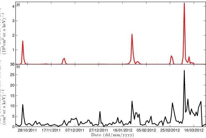
The SEP have a significant ERR for the 350–800 keV pro-tons, which may indicate that the SEPs can penetrate into the magnetosphere to GEO for energies lower than 1 MeV. Fig-ure 2 displays a number of SEP events observed by ACE in the top panel for the energy range 546–761 keV and the daily averaged 350–800 keV protons observed by GOES in the bottom panel, for the period between 18 October 2011 and 26 March 2012. For each of the peaks in SEPs, there is a cor-responding peak in the proton flux at GEO on the same day.
0 1 2 3 4
Dat e ( dd/mm/yyyy)
SE
P
flux
5
4
6
-7
6
1
k
e
V
,
(1
0
4cm
2
sr
s
k
e
V
)
−
1
a)
28/10/2011 17/11/2011 07/12/2011 27/12/2011 16/01/2012 05/02/2012 25/02/2012 16/03/2012 0
5 10 15 20 25 30
Dat e ( dd/mm/yyyy)
GE
O
P
r
o
t
o
n
fl
u
x
3
5
0
-8
0
0
k
e
V
,
(c
m
2
sr
s
k
e
V
)
−
1
[image:5.595.133.467.61.285.2]b)
Fig. 2. Panel (a) displays the daily averaged SEP flux observed by the ACE EPAM for the energy range 546–761 keV and panel (b) shows the daily averaged 350–800 keV protons observed by GOES MAGPD, for the period between 18 October 2011 and 26 March 2012.
However, the 4.2–8.7 MeV and 8.7–14.5 MeV channels have differences between the east and west observations. Both channels have a higher influence from the Dst index for the fluxes inside GEO and also for the IMF-clock angle function. Similar to the inside GEO fluxes, the fluxes outside of GEO are also effected by both Dst and a southward IMF, however, the influence is smaller. Therefore, during geomag-netic storms when the IMF is predominately southward, the probability of SEPs penetrating within the GEO is increased, while the SEPs are more likely to penetrate into the region outside of GEO regardless of IMF direction.
The>350 keV proton fluxes are all very dependent on the current days SEP flux. As such, it will not be possible to pre-dict the next days value because the next days SEP is required for the forecast. Even if the SEPs could be estimated from images from the Sun, it would not be enough since 350 keV protons will take under 8 h to arrive at Earth. Therefore, mod-elling the>350 keV GEO proton fluxes for the purpose of an accurate forecast, will be very difficult. For the <350 keV proton flux the inputs are less reliant on the current days val-ues so a model could be derived for the forecast of the next day fluxes.
5 Conclusions
The ERR study has shown that for energies<800 keV, the main control parameter is the solar wind velocity, showing a similar triangular dependance observed with electron fluxes (Reeves et al., 2011). The lag of the velocity is between 2– 3 days which indicates that the solar wind velocity supplies
the seed population of protons, which is then accelerated over two days to the higher energies.
Another interesting result from the ERR analysis is that, while the solar wind velocity accounts for most of the vari-ance for the 350–800 keV GEO proton fluxes, the SEPs have a significant contribution, 10 % of the ERR. Therefore, the 350–800 keV SEPs may have access to GEO altitudes of the magnetosphere.
For the two highest energy channels (4.2–14.5 MeV), the IMF and Dst index enhance the access of SEPs to altitudes inside and outside of GEO. The fluxes inside GEO had more variance explained by the IMF and Dst compared to the fluxes outside of GEO. Therefore, the probability of SEPs having access to lower altitudes may increase in the case of geomagnetic storms or a southward IMF.
Producing forecast models for the GEO proton flux ener-gies effect by SEP is currently not possible, since to forecast next day’s flux at GEO would also require a forecast of the next day’s SEP flux. However, for the lower energies below 350 keV, the GEO proton fluxes do not rely as much on the current day’s value and therefore it is possible to to derive a forecast model that will estimate the next day’s proton flux at GEO.
Acknowledgements. The authors would like to acknowledge the
financial support from EPSRC, Royal Society collaboration, and ERC. RJB and OAA are grateful for support from ISSI (Bern). The Authors would also like to thank the data providers. OMNIWeb ser-vice for providing the solar wind data, ACE for providing the level 2 EPAM data, and NOAA for the GOES proton flux data at GEO.
References
Balikhin, M. A., Boaghe, O. M., Billings, S. A., and Alleyne, H. S. C. K.: Terrestrial magnetosphere as a nonlinear resonator, Geo-phys. Res. Lett., 28, 1123–1126, 2001.
Balikhin, M. A., Boynton, R. J., Billings, S. A., Gedalin, M., Ganushkina, N., Coca, D., and Wei, H.: Data based quest for so-lar wind-magnetosphere coupling function, Geophys. Res. Lett., 37, L24107, doi:10.1029/2010GL045733, 2010.
Balikhin, M. A., Gedalin, M., Reeves, G. D., Boynton, R. J., and Billings, S. A.: Time scaling of the electron flux increase at geo: The local energy diffusion model vs observations, J. Geophys. Res., 117, A10208, doi:10.1029/2012JA018114, 2012.
Billings, S. A. and Voon, W. S. F.: Correlation based model validity tests for non-linear models, Int. Control J., 44, 235–244, 1986. Billings, S. A., Chen, S., and Korenberg, M. J.: Identification of
mimo non-linear systems using a forward-regression orthogonal estimator, Int. J. Control, 49, 2157–2189, 1989.
Blake, J. B., Martina, E. F., and Paulikas, G. A.: On the access of so-lar protons to the synchronous altitude region, J. Geophys. Res., 79, 1345–1348, doi:10.1029/JA079i010p01345, 1974.
Blake, J. B., Kolasinski, W. A., Fillius, R. W., and Mullen, E. G.: Injection of electrons and protons with energies of tens of mev intol <3 on 24 march 1991, Geophys. Res. Lett., 19, 821–824, doi:10.1029/92GL00624, 1992.
Boaghe, O. M., Balikhin, M. A., Billings, S. A., and Alleyne, H.: Identification of nonlinear processes in the magnetospheric dynamics and forecasting of dst index, J. Geophys. Res., 106, 30047–30066, 2001.
Boynton, R. J., Balikhin, M. A., Billings, S. A., Wei, H. L., and Ganushkina, N.: Using the narmax ols-err algorithm to ob-tain the most influential coupling functions that affect the evo-lution of the magnetosphere, J. Geophys. Res., 116, A05218, doi:10.1029/2010JA015505, 2011.
Boynton, R. J., Balikhin, M. A., Billings, S. A., Reeves, G. D., Ganushkina, N., Gedalin, M., Amariutei, O. A., Borovsky, J. E., and Walker, S. N.: The analysis of electron fluxes at geosyn-chronous orbit employing a narmax approach, J. Geophys. Res. Space Physics, 118, 1500–1513, doi:10.1002/jgra.50192, 2013. Burton, R. K., McPherron, R. L., and Russull, C. T.: An empirical
relationship between interplanetary conditions and dst, J. Geo-phys Res., 80, 4204–4214, 1975.
Daglis, I. A., Thorne, R. M., Baumjohann, W., and Orsini, S.: The terrestrial ring current: Origin, formation, and decay, Rev. Geo-phys., 37, 407–438, doi:10.1029/1999RG900009, 1999. Hanser, F. A.: Eps/hepad calibration and data handbook,
Techni-cal report, Tech. Rep. GOESN-ENG-048D, Assurance Technol. Corp., Carlisle, Mass., 2011.
Horne, R. B., Thorne, R. M., Glauert, S. A., Albert, J. M., Meredith, N. P., and Anderson, R. R.: Timescale for radiation belt electron acceleration by whistler mode chorus waves, J. Geophys. Res., 110, A03225, doi:10.1029/2004JA010811, 2005.
Hudson, M. K., Kotelnikov, A. D., Li, X., Roth, I., Temerin, M., Wygant, J., Blake, J. B., and Gussenhoven, M. S.: Simulation of proton radiation belt formation during the march 24, 1991 ssc, Geophys. Res. Lett., 22, 291–294, doi:10.1029/95GL00009, 1995.
Ivanova, T. A., Kuznetsov, S. N., Sosnovets, E. N., and Tverskaya, L. V.: Dynamics of the latitude limit of penetration of low-energy solar protons into the magnetosphere, Geomagn. Aeron., Engl. Transl., 25, 5–8, 1985.
Kan, J. R. and Lee, L. C.: Energy coupling function and solar wind-magnetosphere dynamo, Geophys. Res. Lett., 6, 577–580, 1979. Leontaritis, I. J. and Billings, S. A.: Input-output parametric models for non-linear systems part i: Deterministic non-linear systems, Int. J. Control, 41, 303–328, 1985a.
Leontaritis, I. J. and Billings, S. A.: Input-output parametric models for non-linear systems part ii: Stochastic nonlinear systems, Int. J. Control, 41, 329–344, 1985b.
Li, X., Roth, I., Temerin, M., Wygant, J. R., Hudson, M. K., and Blake, J. B.: Simulation of the prompt energization and transport of radiation belt particles during the march 24, 1991 ssc, Geo-phys. Res. Lett., 20, 2423–2426, doi:10.1029/93GL02701, 1993. Millan, R. M. and Baker, D. N.: Acceleration of particles to high energies in earth’s radiation belts, Space Sci. Rev., 173, 103–131, doi:10.1007/s11214-012-9941-x, 2012.
Paulikas, G. A. and Blake, J. B.: Penetration of solar protons to synchronous altitude, J. Geophys. Res., 74, 2161–2168, doi:10.1029/JA074i009p02161, 1969.
Reeves, G. D., Morley, S. K., Friedel, R. H. W., Henderson, M. G., Cayton, T. E., Cunningham, G., Blake, J. B., Christensen, R. A., and Thomsen, D.: On the relationship between relativistic elec-tron flux and solar wind velocity: Paulikas and blake revisited, J. Geophys. Res., 116, A02213, doi:10.1029/2010JA015735, 2011. Richard, R. L., El-Alaoui, M., Ashour-Abdalla, M., and Walker, R. J.: Interplanetary magnetic field control of the entry of solar en-ergetic particles into the magnetosphere, J. Geophys. Res., 107, SSH 7–1–SSH 7–20, doi:10.1029/2001JA000099, 2002. Rodriguez, J. V., Onsager, T. G., and Mazur, J. E.: The east-west
effect in solar proton flux measurements in geostationary or-bit: A new goes capability, Geophys. Res. Lett., 37, L07109, doi:10.1029/2010GL042531, 2010.
Roeder, J. L. and Fennell, J. F.: Differential Charging of Satel-lite Surface Materials, IEEE T. Plasma Sci., 37, 281–289, doi:10.1109/TPS.2008.2004765, 2009.
Schulz, M. and Lanzerotti, L. J.: Particle diffusion in the radiation belts, Physics and Chemistry in Space, Berlin: Springer, 1974. Vampola, A. L. and Korth, A.: Electron drift echoes in the
inner magnetosphere, Geophys. Res. Lett., 19, 625–628, doi:10.1029/92GL00121, 1992.