https://doi.org/10.5194/angeo-35-1023-2017 © Author(s) 2017. This work is distributed under the Creative Commons Attribution 3.0 License.
Effects of the planetary waves on the MLT airglow
Fabio Egito1, Hisao Takahashi2, and Yasunobu Miyoshi3
1Centro Multidisciplinar de Bom Jesus da Lapa, Universidade Federal do Oeste da Bahia,
Bom Jesus da Lapa, 47600-000, Brazil
2Aeronomy Division, National Institute for Space Research, São José dos Campos, 12227-010, Brazil
3Department of Earth and Planetary Sciences, Kyushu University, 744 Motooka Nishi-ku Fukuoka, 819-0395, Japan Correspondence to:Fabio Egito ([email protected])
Received: 28 March 2017 – Revised: 18 July 2017 – Accepted: 18 July 2017 – Published: 31 August 2017
Abstract.The planetary-wave-induced airglow variability in the mesosphere and lower thermosphere (MLT) is investi-gated using simulations with the general circulation model (GCM) of Kyushu University. The model capabilities enable us to simulate the MLT OI557.7 nm, O2b(0–1), and OH(6–2)
emissions. The simulations were performed for the lower-boundary meteorological conditions of 2005. The spectral analysis reveals that at middle latitudes, oscillations of the emission rates with the period of 2–20 days appear through-out the year. The 2-day oscillations are prominent in the sum-mer and the 5-, 10-, and 16-day oscillations dominate from the autumn to spring equinoxes. The maximal amplitude of the variations induced by the planetary waves was 34 % in OI557.7 nm, 17 % in O2b(0–1), and 8 % in OH(6–2). The
results were compared to those observed in the middle lati-tudes. The GCM simulations also enabled us to investigate vertical transport processes and their effects on the emission layers. The vertical transport of atomic oxygen exhibits sim-ilar periodic variations to those observed in the emission lay-ers induced by the planetary waves. The results also show that the vertical advection of atomic oxygen due to the wave motion is an important factor in the signatures of the plane-tary waves in the emission rates.
Keywords. Atmospheric composition and structure (air-glow and aurora; middle atmosphere – composition and chemistry) – meteorology and atmospheric dynamics (waves and tides)
1 Introduction
Temporal variations in the airglow emission rates, which originated from the mesosphere and lower thermosphere
(MLT), are important features to understand the photochem-ical and dynamphotochem-ical processes in this region, and they have been extensively studied. Although the airglow is produced mainly thorough chemical reactions that involve minor con-stituents, dynamic processes that change the concentrations of the constituents are important factors in the time varia-tion in the airglow. The airglow temporal variability ranges from short- (a few minutes) to long- (tens of days) term vari-ations because of the solar and anthropogenic effects. In this context, dynamical processes induced by atmospheric waves, such as gravity waves, tides, and planetary waves, play an im-portant role in causing the airglow variability. Historically, the Krassovsky parameter (Krassovsky, 1972) has been used to indicate the gravity-wave-induced perturbations in the air-glow. Ground-based observations showed diurnal and semid-iurnal variations in the airglow, which were explained by at-mospheric tides (Wiens and Weill, 1972; Fukuyama, 1976). Using satellite observations, Shepherd et al. (2006) further studied the effect of tidal oscillations on the airglow vari-abilities. Combined observational and modeling studies have also helped to understand the interaction and effect of these waves in the emissions (Walterscheid and Schubert, 1995; Yee et al., 1997; Snively et al., 2010; Liu et al., 2008).
planetary-wave activity in the airglow was extended to cover latitudes from the pole to the equator. In the arctic region, the 5-day, 10-day, and 16-day periodic variations in the emis-sion rates have been attributed to the Rossby normal modes (Sivjee et al., 1994; Espy et al., 1996, 1997). In the middle latitudes, Lopez-Gonzalez et al. (2009) presented an exten-sive statistical study about the occurrence and characteristics of planetary-wave signatures in the hydroxyl and molecular oxygen airglow intensities and the respective rotational tem-peratures. In the equatorial region, Takahashi et al. (2002) and Buriti et al. (2005) reported 3–4-day periodic oscillations in the airglow intensities, which were attributed to the 3.5-day ultra-fast Kelvin wave. Measurements by the WINDII in-strument (Wind Imager Interferometer) on board the UARS satellite (Upper Atmosphere Research Satellite) enabled the observation of planetary-scale structures in the airglow emis-sion rates (Shepherd et al., 1993). From this dataset, Ward et al. (1997) retrieved the signature of 2-day waves in the atomic oxygen green line. Other satellite-borne studies (e.g., Liu and Shepherd, 2006; Xu et al., 2010) have reported lon-gitudinal variations in the MLT airglow and associated them with the passage of planetary-scale waves through the emis-sion layers.
Many previous studies on the airglow variability have fo-cused on observing the planetary-wave activity, but modeling studies have not been fully explored. Walterscheid and Schu-bert (1995) investigated the effects of the planetary-wave normal modes on the OH emission using the Krassosvky theory for an isothermal, inviscid, and windless atmosphere. Lichstein et al. (2002) used a one-dimensional model to sim-ulate the 3.5-day oscillation of the airglow intensities that Takahashi et al. (2002) observed. They concluded that the observed oscillation was consistent with an ultra-fast Kelvin wave.
Observational evidence and numerical simulations have indicated that vertical transport is mainly responsible for the observed airglow variations (Shepherd et al., 2006; Liu et al., 2008). Cho and Shepherd (2006) argued that the un-derlying process behind both short- and long-term airglow variations most likely involve vertical motions, which act on the atomic oxygen transport. Combining atomic oxy-gen OI557.7 nm emission measurements by WINDII with TIME-GCM (Thermosphere–Ionosphere–Mesosphere Elec-trodynamics general circulation model) simulations, Liu et al. (2008) showed that the daily airglow variability is a straightforward result of the vertical transport of atomic oxy-gen due to the tidal vertical motions. Concerning planetary waves, Ward et al. (1997) pointed out that the vertical trans-port of atomic oxygen is responsible for the observed 2-day variations in the atomic oxygen green line measured by WINDII. Nevertheless, it is unclear whether their proposed mechanism holds for longer-period waves such as 5-, 10-, and 16-day planetary waves.
Although the activity and some characteristics of the in-duced airglow variations by planetary-scale waves are
rela-tively well known, their effects on the composition of con-stituents such as atomic oxygen and the consequent airglow variations are not well understood. In the present study, we used the Kyushu general circulation model to simulate air-glow emissions coming from the MLT region to investigate the activity of the planetary waves. Then, we used the sim-ulations to investigate the mechanisms responsible for the planetary-wave-induced variations in the airglow emissions.
2 Data and simulation model
In this study, we numerically simulated the temporal varia-tion in the airglow emission rates by using the general cir-culation model of Kyushu University (hereafter abbreviated as Kyushu GCM). The Kyushu GCM is a global spectral model, which was originally developed as a meteorological and climate model and extended to the middle and upper at-mosphere at Kyushu University (Miyahara et al., 1993). The model contains a vertical extension from the ground to the exobase (approximately 500 km), where the set of non-linear equations for the zonal and meridional momentum budget, thermodynamics, continuity, and hydrostatic is solved at con-stant pressure levels. The model incorporates a full set of appropriate physical processes for the troposphere, strato-sphere mesostrato-sphere, and thermostrato-sphere. The effects of the Earth surface topography, contrast between land and sea tem-peratures, and moist convection are considered. The model also includes the assimilation of the meteorological reanaly-sis data from the JRA-25 project (25-year Japanese ReAnaly-sis) (Onogi et al., 2005). Using a nudging technique, the solu-tions of the equasolu-tions are forced towards reanalysis data from the ground to approximately 30 km in altitude. The Kyushu GCM has a spectral model of T42, which corresponds to a 2.8◦ horizontal resolution in longitude and latitude. It con-tains 75 vertical layers with a vertical resolution of 0.4-scale height above the troposphere, which corresponds to approxi-mately 2 km in the MLT heights. Further details can be found elsewhere (Miyoshi et al., 1999, 2003, 2006).
2.1 Airglow photochemistry
tidal variations in the O(1S) and OH emissions. The approach used to simulate the airglow intensity variability in differ-ent dynamical processes depends on the characteristics of the model and the purpose of the study. To simulate airglow emissions by using the Kyushu GCM, we used the steady-state photochemistry approach. In this case, we have consid-ered the photochemical balance between the production and loss processes to simulate the emissions rates. Dynamical ef-fects of the waves were incorporated into the constituents and temperature, which was originally calculated in the model. In this study, we simulated the OI557.7 nm (hereafter OI5577), O2b(0–1) band (hereafter O2b(0–1)), and OH (6–2) band
(hereafter OH(6–2)) MLT airglow emissions, which enabled further comparison with ground-based observations. In the next section, we describe the basic photochemistry of each emission.
2.1.1 The OI5577 and O2b(0–1) emissions
It is well established that the excited state responsible for the OI5577 green line emission in the MLT is produced by the two-step Barth’s mechanism (Barth, 1961). In this mecha-nism a three-body recombination reaction between two oxy-gen atoms in the presence of a third body produces an ex-cited state of the molecular oxygen, which subsequently re-acts with other atomic oxygen and produces the excited state:
O+O+M→O2∗+M, (1)
O2∗+O→O(1S)+O2, (2)
whereM=O2+N2is the atmospheric third body and O2∗
is an intermediate excited state.
The production mechanism of the excited state of the O2b(0–1) atmospheric band is similar to that of the OI5577
green line, but in the second step, the energy is transferred from the O∗2excited state to the molecular oxygen instead of the atomic oxygen. The reactions are as follows:
O+O+M→O2∗+M, (3)
O2∗+O2→O2
b16g++O2. (4)
Loss processes for O(1S) and O2(b16g+)occur via quenching
and radiative decay and must be considered for the O∗2. Considering the photochemical balance equations pre-sented by McDade et al. (1986), the volumetric emission rates of the OI5577 and O2b(0–1) can be calculated as
VOI5577=
A5k1[O]3([N2]+[O2])
(A6+k5[O2]) CO2 0[O
2]+CO[O]
, (5)
VO2(0−1)=
A1k1[O2] [O]2([N2]+[O2])
A2+k2O2[O2]+kN22[N2]
CO2[O2]+CO[O]
, (6) where A1,A2,A5, andA6 are the transition probabilities,
k1,k2,k2O2, andk N2
2 are the reaction coefficients, and C 0 O2, C0O, CO2, and CO are constants, which were obtained from McDade et al. (1986) and references therein.
2.1.2 The OH emission
The main source of the airglow OH Meinel bands is the exothermic reaction between ozone and hydrogen (Bates et al., 1950):
H+O3→OH∗(υ≤9)+O2, (7)
whereυis the vibrational level of the OH molecule. Lower vibrational levels are also populated by collisional and radiative cascade. The loss processes include quenching and radiative relaxation. In the nighttime MLT, the ozone is produced in the recombination reaction O2+O+M→
O3+M and destroyed in Eq. (7), which is in
photochem-ical balance (Brassuer et al., 2005). Considering this and the other photochemical equations presented by Makhlouf et al. (1995), the volumetric emission rate for the OH(6–2) band can be expressed as
VOH(6−2)=
A(6,2)f (6)k1[O][O2][M]
+P9υ=7A(υ,6)[OH(υ)]+P9υ=7[OH(υ)] (
P Mi
kQi2 (υ,6)[Mi] )
X
Mi kMi
L (6)[Mi]+A (6) ,
(8)
wherek1 is the reaction coefficient for Eq. (7); f(6) is the
quantum yield for the vibrational level 6;A(6,2),A(υ,6), and A(6) are the Einstein transition probabilities;kQi
2 andk Mi L
are the collisional cascade production and quenching coeffi-cients, respectively, between the OH excited states and other species (primarily O2and N2).
To calculate the OH(6–2) band from Eq. (8), we have used the reaction coefficients and other parameters from Makhlouf et al. (1995), except the Einstein transitions probabilities, which we obtained from Langhoff et al. (1986).
2.2 Airglow simulations
3 Results and discussion 3.1 Planetary-wave signatures
Temporal variations in the OI5577, O2b(0–1), and OH(6–
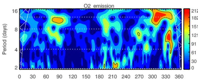
2) emission rates were simulated as described in Sect. 2.1. Planetary-wave-induced variations in the MLT airglow emis-sions have been reported from middle-latitude ground-based observations (e.g., Takahashi et al., 2013; Lopez-Gonzalez et al., 2009). To study the effect of the planetary-wave activ-ity on the airglow and to compare it with the ground-based MLT airglow measurements, we initially analyzed the vari-ability in the emissions at 43◦N and 143◦E, which is the nearest model grid point to the Rikubetsu airglow observa-tory at (43.5◦N, 143.8◦E). Dominant periodic oscillations were identified in the averaged airglow integrated intensi-ties. Figure 1 shows the wavelet spectrum of the simulated O2b(0–1) emission with the assimilated data in 2005. To
calculate the power spectrum, the Morlet wavelet transform was used (Torrence and Compo, 1998). Periodic oscillations near 5, 10, and 16 days appear intermittently throughout the year. The wave activity is more intense during the autumn and winter months. From the spring equinox to the autumn equinox, the wave activity decreases. In the present case, there is some activity related to the 2-day wave after the sum-mer solstice. Longer-period oscillations, i.e., 10- and 16-day oscillations, have significant spectral energy before and after the spring and autumn equinoxes, respectively. The spectrum shows three well-defined periodic oscillations at the periods near 5, 10, and 16 days. The 10-day oscillation appears on approximately day 90 (March/April). Between days 300 and 330 (November), there is an oscillation whose spectral en-ergy spreads from 10 to 16 days and is centered at 12 days. Immediately after day 330, there is also a well-defined 6.5-day oscillation. The spectral contents of the OI5577 and OH(6–2) emissions (not shown here) show essentially identi-cal features to those in Fig. 1 for the O2b(0–1) emission. The
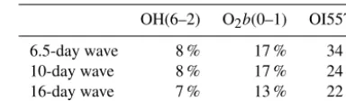
amplitudes of variation in these emissions appear indepen-dent from the period of oscillation (6.5–16 days). However, these three emissions show different amplitudes of variation against the passage of waves. Relative to the mean inten-sity, the amplitudes are 7–8 % in the OH(6–2) emission, 13– 17 % in theO2b(0–1) emission, and 22–34 % in the OI5577
emission. Table 1 shows the relative amplitudes induced by the 6.5-, 10-, and 16-day planetary-scale waves in the emis-sions. The relative amplitudes of the waves for different pe-riods systematically increase from the OH(6–2) to O2b(0–1)
and to OI557.7 nm emissions. Ground-based observations of planetary-wave signatures in the airglow also depict a simi-lar scenario (e.g., Lopez-Gonzales et al., 2009; Takahashi et al., 2013). Such behavior may be related to the dependence of each emission on the atomic oxygen concentration, which is approximately linear, squared, and cubic in the OH(6–2), O2b(0–1), and OI557.7 nm emissions, respectively, as shown
[image:4.612.332.524.97.153.2]in Eqs. (5), (6), and (8).
Table 1.Relative amplitudes induced by the 6.5-, 10-, and 16-day waves in the OH(6–2), O2b(0–1), and OI5577 emissions.
OH(6–2) O2b(0–1) OI5577
6.5-day wave 8 % 17 % 34 %
10-day wave 8 % 17 % 24 %
16-day wave 7 % 13 % 22 %
The planetary-wave activity in the MLT region varies as a function of time and space, which reflects the variability in the sources and conditions of propagation. Signatures of such periodic oscillations are clearly observed in the wind structures. For the middle latitudes, waves with longer pe-riods of 10 and 16 days are common features in autumn and winter seasons, 5-day waves frequently appear around equinoxes, and 2-day waves intensify in the summer (Chshy-olkova et al., 2005; Jiang et al., 2005, 2008). For the air-glow and planetary-wave observations, López-Gonzalez et al. (2009) extensively investigated the planetary-wave ac-tivity in the middle-latitude MLT based on ground mea-surements of the airglow at the Sierra Nevada observatory (37.06◦N, 3.38◦W). Their analysis, which covered almost 10 years (1998–2007), showed 10- and 16-day oscillations that peaked in autumn and winter and 5-day oscillations with maximum intensifications near the equinoxes and strong quasi-2-day oscillations in winter and summer. By analyzing the airglow and wind data at Rikubetsu (43.5◦N, 143.8◦E) and Wakkanai (45.4◦N, 141.7◦E), respectively, Takahashi et al. (2013) showed a similar scenario. Large amplitudes of os-cillation of the airglow intensities were reported in these two studies. For 10- and 16-day waves, Takahashi et al. (2013) reported amplitudes of up to 57 % in the OI5577, 51 % in the O2b(0–1), and 29 % in the OH(6–2). The amplitudes of
os-cillation reported by López-Gonzalez et al. (2009) also pre-sented higher amplitudes of oscillation than our values here. Despite the difference in the magnitudes, the amplitudes pre-sented here show identical behavior in each emission, i.e., the amplitudes in the OI5577 and O2(0–1) are
systemati-cally higher than that in OH(6–2). Therefore, the planetary-wave signatures in the MLT airglow simulated by the Kyushu GCM essentially exhibit a similar seasonal variation to those in airglow and wind measurements. This finding indicates that the Kyushu GCM reproduces well the planetary-wave activity in the airglow and some of its features in the MLT. 3.2 The 10-day wave
-1
-3 -3 -1 -3 -1
[image:5.612.101.497.67.209.2](a) (b) (c)
Figure 1.Time–altitude distribution of the volumetric emission rates of the OI5577(a), O2b(0–1)(b), and OH(6–2)(c)at 43◦N and 143◦E. Time interval covers March and April for 2005 simulations.
Figure 2.Wavelet spectrum of the nightly mean column intensity of the O2b(0–1) emission rates simulated by the Kyushu GCM at 43◦N and 143◦E from January to December 2005.
of the OI5577, O2b(0–1), and OH(6–2) emissions at 43◦N
and 143◦E, which is the closest grid point to the Rikubetsu airglow observatory. All of the three emissions exhibit a clear variation of approximately 10 days that lasted approximately two cycles, and the first maximum was between days 75 and 80. The 10-day oscillation exhibits relatively distinct mag-nitudes in each emission. In the OI5577 emission, the VER is drastically reduced during the minimum phase. The reduc-tion is gradually lower in the O2(0–1) and OH (6–2) emission
rates. From the harmonic analysis, we estimated the ampli-tudes of the 10-day oscillation relative to the mean value dur-ing the studied period. To compare with ground-based obser-vations, we integrated the emission rates to obtain the nightly averaged intensities. The integrated intensities are expressed in Rayleigh (R). The amplitude perturbations are 24 % in the OI5577, 17 % in the O2b(0–1), and 8 % in the OH(6–2).
The 10-day oscillations are primarily associated with the 10-day Rossby normal mode. To investigate the zonal struc-ture of this oscillation, we applied the space–time spectral analysis (Hayashi, 1971), which simultaneously reveals the zonal wavenumber and the frequency (period) in the data. Figure 3 shows space–time spectra for the simulated OI5577,
O2b(0–1), and OH (6–2) integrated intensities at 43◦N. The
data correspond to the interval of days 75–110. A spectral peak that corresponds to the zonal wavenumber−1 and a period of approximately 10 days are clearly observed in all three emissions. The negative (positive) zonal wavenumber corresponds to the westward (eastward) propagation. There-fore, the 10-day oscillation in the airglow exhibits character-istics of a westward-propagating wave with zonal wavenum-ber 1. In addition to this wave, there is also a secondary peak related to a 6.5-day westward-propagating wave with a zonal wavenumber of 1. Interestingly, the 6.5-day wave amplitude is particularly strong in the OH(6–2) emission. Its amplitude is similar to that of the 10-day wave. The signature of the 6.5-day wave is observed in the emission rates in Fig. 2 on approximately day 90, when there is a split during the max-imum phase of the 10-day wave. The superposition of the 10-day and 6.5-day waves is more pronounced in the OH(6– 2) emission, which may suggest a vertical damping of the 6.5-day wave.
[image:5.612.128.466.260.399.2]ampli-Figure 3.Space–time spectra of the OI5577(a), O2b(0–1)(b), and OH(6–2)(c)emissions at 43◦N.
Figure 4.Latitudinal structure of the zonal wavenumber 1, westward-propagating 10-day wave.
tude are shown in Fig. 4. The data corresponds to the inter-val of days 75–110 around the March equinox. In general, the amplitude of the 10-day wave peaks at middle latitudes and minimizes at the equator and poles. The wave also ex-hibits an asymmetric amplitude distribution around the equa-tor. Comparing the amplitudes between the Northern and Southern Hemispheres, we notice that those in the OH(6–2) and O2b(0–1) emissions are higher in the Northern
Hemi-sphere, whereas the amplitudes of OI5577 are higher in the Southern Hemisphere. On the other hand, the amplitudes of the OI5577 emission are higher in the Southern Hemisphere. In addition, the wave amplitude structure of the OH emission is slightly distorted, and its zero level is displaced by approx-imately 30◦ from the equator. The 10-day wave, which is normally associated with the free Rossby normal mode (1, −3), is the first asymmetric mode from classical planetary-wave theory (Forbes, 1995). Its horizontal structure in den-sity, temperature, and vertical and zonal wind is antisymmet-ric with respect to the equatorial node and peaks at mid-dle latitudes. The characteristics of the horizontal structure of the presented 10-day wave here are similar to the afore-mentioned characteristics, which indicates that the airglow variations in March/April are consistent with a signature of the normal mode (1, −3). The 10-day oscillation identified in this work was observed in the airglow and wind mea-surements by Takahashi et al. (2013), which reinforces the model’s capability to reproduce the planetary-wave activity in the MLT airglow.
3.3 Airglow response to planetary waves
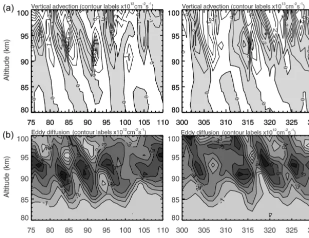
The comparison of the day-to-day variations in the MLT airglow intensities between the observation and the model simulation shows that the Kyushu GCM can reproduce the planetary-wave activity in the MLT airglow well. Further-more, it is well known that the vertical transport process, par-ticularly that of atomic oxygen, has an important role in the airglow intensity variability (e.g., Cho and Shepherd, 2006). Thus, a diagnostic post-processing analysis was performed to evaluate the importance of the vertical transport of atomic oxygen via eddy diffusion and advection due to the wave wind field. The vertical transport of atomic oxygen via ad-vection and eddy diffusion was calculated as follows:
fadv=w[O], (9)
feddy= −K[N2]
d dz
[O]
[N2]
, (10)
wherew is the vertical velocity, [O] and [N2] are,
respec-tively, the atomic oxygen and molecular nitrogen concentra-tions,zis the vertical coordinate, and K is the eddy diffusion coefficient, which was obtained from Chen (2012).
[image:6.612.85.518.226.342.2](a)
[image:7.612.145.454.67.305.2](b)
Figure 5.Daily mean transport of atomic oxygen by vertical advection(a)and eddy diffusion(b)at 43◦N and 143◦E. Contour labels ×1013cm−2s−1for vertical advection and×1012cm−2s−1for eddy diffusion.
-1
-3 -3-1 -3 -1
(a) (b) (c)
Figure 6.Time–altitude distribution of the volumetric emission rates of the OI5577(a), O2b(0–1)(b), and OH(6–2)(c)at 43◦N and 143◦E. Time interval covers October and November for 2005 simulations.
indicate the downward and upward transports, respectively. During both intervals, the vertical transport of atomic oxy-gen by advection and eddy diffusion exhibits periodic varia-tions, which are associated with the 10-day wave like those observed in the airglow. This feature indicates a direct rela-tionship between the vertical transport of atomic oxygen due to the 10-day wave and the correspondent airglow-induced variability. Despite similar time variabilities, the advection and eddy diffusion present distinct characteristics. The ad-vection changes direction (alternating between upward and downward flux), whereas the eddy diffusion is predominantly downward. Furthermore, the magnitudes of eddy diffusion are approximately 10 times lower than the magnitude of ver-tical advection.
To understand the relationship between the vertical trans-port of atomic oxygen and the airglow periodic oscillations, we compared their temporal variation. Figure 2 shows that emission rates are maximal on approximately days 80, 90, and 100 and minimal on approximately days 85 and 95. Comparing the temporal variability in the emissions rates shown in Fig. 2 with the vertical transport processes shown in Fig. 5, we note that for most of the altitudes, the high emis-sion rates match the downward flux due to vertical advection and intensifications in the downward eddy diffusion. Mean-while, the low emission rates are related to the upward flux due to vertical advection and decreasing eddy diffusion. Fig-ure 6 shows the volume emission rates of OH(6–2), O2b(0–
[image:7.612.105.495.353.494.2]cor-respond to the interval when 5- and 16-day oscillations were observed. This figure shows that the variability in the air-glow emission rates and vertical transport of atomic oxygen is similar to that for the 10-day wave; i.e., high emission rates are related to the downward advection and increasing down-ward eddy diffusion and vice versa. The vertical wind gen-erated by wave propagations primarily drives the vertical ad-vection. Therefore, the vertical motion induced by the wave wind field is the primary source of the observed periodic 5-, 10-, and 16-day variations observed in the airglow emissions. As noted by Liu et al. (2008), the eddy diffusion contributes to the background intensities by transporting atomic oxygen downward, and the vertical advection explains the time vari-ability in the emissions due to wave-induced vertical motion. The airglow variability as a result of vertical motions has been attributed to quasi-adiabatic processes that conserve the atomic oxygen mixing ratio (Ward at al., 1994, 1997). In this case, when the atomic oxygen mixing ratio increases with altitude in the MLT, the downward motion brings down the atomic-oxygen-rich air, and then emission rates increase. In contrast, in the upward motion, the proportionally atomic-oxygen-poor air is moved up, and then emission rates de-crease. The additional effect of this quasi-adiabatic process is to increase and decrease the temperature of the air dur-ing the downward and upward displacements, respectively. Although, the airglow variability is the result of many physi-cal and chemiphysi-cal processes that occur together, the evidence presented here indicates that the airglow response to the pen-etration of planetary waves in the emission layers is primar-ily driven by the vertical transport of atomic oxygen. Ward et al. (1997) explained the enhancement of airglow emis-sion rates with the vertical advection induced by 2-day plane-tary waves instead of the atomic-oxygen mixing ratio caused by the wave-breaking process. Our simulation model results also indicate that the longer-period planetary waves (5-, 10-, 16-day) may produce vertical advection and result in the air-glow day-to-day variability.
4 Conclusions
In this study, we investigated the effects of planetary waves on the MLT airglow by simulating the OH(6–2), O2b(0–
1), and OI5577 MLT emissions using the general circula-tion model of Kyushu University. Periodic variacircula-tions of 2– 20 days in the simulated emissions were observed over the course of the year. At middle latitudes, the wave activity intensifies from autumn to spring equinoxes, where the 5-, 10-, and 16-day waves dominate the airglow variability. The planetary-wave activity in the simulated airglow exhibits a similar seasonal variability to that observed in the wind and airglow, which indicates that the model can reproduce the airglow variability induced by the planetary waves. The am-plitudes of variation induced by the 5-, 10-, and 16-day plan-etary waves are 7–8 % in the OH(6–2) emission, 13–17 %
in the O2b(0–1) emission, and 22–34 % in the OI5577
emis-sion. It is revealed that the vertical transport of atomic oxy-gen by vertical advection and eddy diffusion oxy-generated by the 5-, 10-, and 16-day planetary waves is responsible for the observed day-to-day variabilities of the MLT airglow.
Data availability. The model data used in this study are available upon request to the authors.
Competing interests. The authors declare that they have no conflict of interest.
Acknowledgements. We thank the Conselho Nacional de
De-senvolvimento Científico e Tecnológico-CNPq (processes
no. 141813/2009-1, 200228/2011-0, and 305461/2015-0) for the financial support for the present study. The authors also thank Kazuo Shiokawa at the Institute of Space-Earth Environmental Research (ISEE), Nagoya University, who provided the airglow data from Rikubetsu, Japan.
The topical editor, Keisuke Hosokawa, thanks two anonymous referees for help in evaluating this paper.
References
Angelatis i Coll, M. and Forbes, J. M.: Dynamical influences on atomic oxygen and 5577Å emission rates in the lower thermo-sphere, Geophys. Res. Lett., 25, 461–464, 1998.
Barth, C. A.: The 5577-angstrom airglow, Science, 134, 1426–1430, 1961.
Brasseur, G. P. and Solomon, S.: Aeronomy of the Middle Atmo-sphere, 3th Edn., Springer, Dordrecht, 2005.
Buriti, R. A., Takahashi, H., Lima, L. M., and Medeiros, A. F. Equa-torial planetary waves in the mesosphere observed by airglow periodic oscillations, Adv. Space Res., 35, 2031–2036, 2005. Chen, Y. W.: Analyses of fast and ultrafast kelvin waves simulated
by the Kyushu-GCM: wave behavior and excitation sources, PhD Thesis – Kyushu University, Fukuoka-Japan, 119 pp., 2012. Cho, Y. M. and Shepherd, G. G.: Correlation of airglow
tem-perature and emission rate at Resolute Bay (74.68◦N), over four winters (2001–2005), Geophys. Res. Lett., 33, L06815, https://doi.org/10.1029/2005GL025298, 2006.
Chshyolkova, T., Manson, A. H., and Meek, C. E.: Climatology of the quasi two-day wave over Saskatoon (52◦N, 107◦W): 14 Years of MF radar observations, Adv. Space Res., 35, 2011– 2016, 2005.
Espy, P. J. and Witt, G.: Observation of a quasi 16-day oscillation in the polar summer mesospheric temperature, Geophys. Res. Lett., 23, 1071–1074, 1996.
Espy, P. J., Stegman, J., and Witt, G.: Interannual variations of the quasi-16-day oscillation in the polar summer mesospheric tem-perature, J. Geophys. Res.-Atmos., 102, 1983–1990, 1997. Forbes, J. M.: Tidal and planetary waves, in: The Upper Mesosphere
Fukuyama, K.: Airglow variations and dynamics in the lower ther-mosphere and upper mesosphere – I. Diurnal variation and its seasonal dependency, J. Atmos. Terr. Phys., 38, 1279–1287, 1976.
Hayashi, Y.: A generalized method of resolving disturbances into progressive and retrogressive waves by space Fourier and time cross-spectral analyses, J. Meteorol. Soc. Jpn., 49, 125–128, 1971.
Horinouchi, T.: Simulated breaking of convectively generated mesoscale gravity waves and airglow modulation, J. Atmos. Terr. Phys., 66, 755–767, 2004.
Jiang, G., Xiong, J., Wan, W., Ning, B., Liu, L., Vincent, R. A., and Reid, I.: The 16-day waves in the mesosphere and lower ther-mosphere over Wuhan (30.6◦N, 114.5◦E) and Adelaide (35◦S, 138◦E), Adv. Space Res., 35, 2005–2010, 2005.
Jiang, G., Xiong, J., Wan, W., Ning, B., and Liu, L.: Observation of 6.5-day waves in the MLT region over Wuhan, J. Atmos. Sol.-Terr. Phys., 70, 41–48, 2008.
Krassovsky, V. I.: Infrasonic variations of OH emission in the upper atmosphere, Ann. Geophys., 28, 739–746, 1972.
Langhoff, S. R., Werner, H. J., and Rosmus, P.: Theoretical Transition-Probabilities for the Oh Meinel System, J. Mol. Spec-trosc., 118, 507–529, 1986.
Lichstein, G. S., Forbes, J. M., Coll, M. A. I., Takahashi, H., Gobbi, D., and Buriti, R. A.: Quasi-3-day kelvin wave and the OI(5577 angstrom), OH(6,2) Meinel, and O-2(0,1) emissions, Geophys. Res. Lett., 29, 1043–1046, 2002.
Liu, A. Z. and Swenson, G. R.: A modeling study of O-2 and OH airglow perturbations induced by atmospheric gravity waves, J. Geophys. Res.-Atmos., 108, D44151, https://doi.org/10.1029/2002JD002474, 2003.
Liu, G. and Shepherd, G. G.: An empirical model for the altitude of the OH nightglow emission, Geophys. Res. Lett., 33, L09805, https://doi.org/10.1029/2005GL025297, 2006.
Liu, G. P., Shepherd, G. G., and Roble, R. G.: Seasonal variations of the nighttime O(1S) and OH airglow emis-sion rates at mid-to-high latitudes in the context of the large-scale circulation, J. Geophys. Res.-Space, 113, A06302, https://doi.org/10.1029/2007JA012854, 2008.
López-González, M. J., Rodríguez, E., García-Comas, M., Costa, V., Shepherd, M. G., Shepherd, G. G., Aushev, V. M., and Sargoytchev, S.: Climatology of planetary wave type oscilla-tions with periods of 2–20 days derived from O2atmospheric and OH(6–2) airglow observations at mid-latitude with SATI, Ann. Geophys., 27, 3645–3662, https://doi.org/10.5194/angeo-27-3645-2009, 2009.
Makhlouf, U. B., Picard, R. H., and Winick, J. R.: Photochemical-Dynamical Modeling of the Measured Response of Airglow to Gravity-Waves, 1. Basic Model for Oh Airglow, J. Geophys. Res.-Atmos., 100, 11289–11311, 1995.
Makhlouf, U. B., Picard, R. H., Winick, J. R., and Tuan, T. F.: A model for the response of the atomic oxygen 557.7 nm and the OH Meinel airglow to atmospheric gravity waves in a realistic atmosphere, J. Geophys. Res.-Atmos., 103, 6261–6269, 1998. McDade, I. C. and Llewellyn, E. J.: The excitation of O(1S) and
O-2 bands in the nightglow – a brief review and preview, Can. J. Phys., 64, 1626–1630, 1986.
Miyahara, S., Yoshida, Y., and Miyoshi, Y.: Dynamic coupling be-tween the lower and upper-atmosphere by tides and gravity-waves, J. Atmos. Terr. Phys., 55, 1039–1053, 1993.
Miyoshi, Y.: Numerical simulation of the 5-day and 16-day waves in the mesopause region, Earth Planets Space, 51, 763–772, 1999. Miyoshi, Y. and Fujiwara, H.: Day-to-day variations of
mi-grating diurnal tide simulated by a GCM from the ground surface to the exobase, Geophys. Res. Lett., 30, 1789, https://doi.org/10.1029/2003GL017695, 2003.
Miyoshi, Y. and Fujiwara, H.: Excitation mechanism of in-traseasonal oscillation in the equatorial mesosphere and lower thermosphere, J. Geophys. Res.-Atmos., 111, D14108, https://doi.org/10.1029/2005JD006993, 2006.
Onogi, K., Koide, H., Sakamoto, M., Kobayashi, S., Tsutsui, J., Hat-sushika, H., Matsumoto, T., Yamazaki, N., Kamahori, H., Taka-hashi, K., Kato, K., Oyama, R., Ose, T., Kadokura, S., and Wada, K.: JRA-25: Japanese 25-year re-analysis project – progress and status, Q. J. Roy. Meteor. Soc., 131, 3259–268, 2005.
Shepherd, G. G., Thuillier, G., Solheim, B. H., Chandra, S., Cogger, L. L., Duboin, M. L., Evans, W. F. J., Gattinger, R. L., Gault, W. A., Herse, M., Hauchecorne, A., Lathuilliere, C., Llewellyn, E. J., Lowe, R. P., Teitelbaum, H., and Vial, F.: Longitudinal struc-ture in atomic oxygen concentrations observed with WINDII on UARS, Geophys. Res. Lett., 20, 1303–1306, 1993.
Shepherd, G. G., Cho, Y. M., Liu, G. P., Shepherd, M. G., and Roble, R. G.: Airglow variability in the context of the global meso-spheric circulation, J. Atmos. Sol.-Terr. Phys., 68, 2000–2011, 2006.
Sivjee, G. G., Walterscheid, R. L., and Mcewen, D. J. Planetary wave disturbances in the arctic winter mesopause over eureka (80◦N), Planet. Space Sci., 42, 973–986, 1994.
Snively, J. B., Pasko, V. P., and Taylor, M. J.: OH and OI air-glow layer modulation by ducted short-period gravity waves: Ef-fects of trapping altitude, J. Geophys. Res.-Space, 115, A11311, https://doi.org/10.1029/2009JA015236, 2010.
Takahashi, H., Buriti, R. A., Gobbi, D., and Batista, P. P.: Equato-rial planetary wave signatures observed in mesospheric airglow emissions, J. Atmos. Sol.-Terr. Phys., 64, 1263–1272, 2002. Takahashi, H., Shiokawa, K., Egito, F., Murayama, Y., Kawamura,
S., and Wrasse, C. M.: Planetary wave induced wind and airglow oscillations in the middle latitude MLT region, J. Atmos. Sol.-Terr. Phys., 98, 97–104, 2013.
Teitelbaum, H., Massebeuf, M., Fellous, J. L., Petitdidier, M., Christophe, J., and Blanco, F.: Simultaneous Measurements of Meteor Winds and Green Line Intensity Variations – Gravity-Waves and Planetary-Gravity-Waves, J. Geophys. Res.-Space, 86, 7767– 7770, 1981.
Torrence, C. and Compo, G. P.: A practical guide to wavelet analy-sis, B. Am. Meteorol. Soc., 79, 61–78, 1998.
Vargas, F., Swenson, G., Liu, A., and Gobbi, D.: O(S-1), OH, and O-2(b) airglow layer perturbations due to AGWs and their im-plied effects on the atmosphere, J. Geophys. Res.-Atmos., 112, D14102, https://doi.org/10.1029/2006JD007642, 2007. Walterscheid, R. L. and Schubert, G.: Dynamical-chemical model
of fluctuations in the OH airglow driven by migrating tides, sta-tionary tides, and planetary-waves, J. Geophys. Res.-Space, 100, 17443–17449, 1995.
the mesospheric o(s−1) emission peak intensity and height, and temperature at 98 km using WINDII data, Adv. Space Res., 14, 57–60, 1994.
Ward, W. E., Solheim, B. H., and Shepherd, G. G.: Two day wave induced variations in the oxygen green line volume emission rate: WINDII observations, Geophys. Res. Lett., 24, 1127–1130, 1997.
Ward, W. E., Oberheide, J., Riese, M., Preusse, P., and Offermann, D.: Tidal signatures in temperature data from CRISTA 1 mission, J. Geophys. Res.-Atmos., 104, 16391–16403, 1999.
Wiens, R. H. and Weill, G.: Diurnal, annual and solar cycle vari-ations of hydroxyl and sodium nightglow intensities in the Europe–Africa sector, Planet. Space Sci., 21, 1011–1027, 1973.
Xu, J., Smith, A. K., Jiang, G., Gao, H., Wei, Y., Mlynczak, M. G., and Russell III, J. M.: Strong longitudinal varia-tions in the OH nightglow, Geophys. Res. Lett., 37, L21801, https://doi.org/10.1029/2010GL043972, 2010.