www.ann-geophys.net/34/1085/2016/ doi:10.5194/angeo-34-1085-2016
© Author(s) 2016. CC Attribution 3.0 License.
Deduction of the rates of radial diffusion of protons from the
structure of the Earth’s radiation belts
Alexander S. Kovtyukh
Skobeltsyn Institute of Nuclear Physics, Moscow State University, 119899, Moscow, Russia Correspondence to:Alexander S. Kovtyukh ([email protected])
Received: 12 May 2016 – Revised: 31 October 2016 – Accepted: 1 November 2016 – Published: 23 November 2016
Abstract. From the data on the fluxes and energy spectra of protons with an equatorial pitch angle of α0≈90◦
dur-ing quiet and slightly disturbed (Kp≤2) periods, I directly calculated the value DLL, which is a measure of the rate
of radial transport (diffusion) of trapped particles. This is done by successively solving the systems (chains) of inte-grodifferential equations which describe the balance of radial transport/acceleration and ionization losses of low-energy protons of the stationary belt. This was done for the first time. For these calculations, I used data of International Sun– Earth Explorer 1 (ISEE-1) for protons with an energy of 24 to 2081 keV at L=2–10 and data of Explorer-45 for pro-tons with an energy of 78.6 to 872 keV at L=2–5. Ioniza-tion losses of protons (Coulomb losses and charge exchange) were calculated on the basis of modern models of the plas-masphere and the exosphere. It is shown that for protons withµfrom∼0.7 to∼7 keV nT−1atL≈4.5–10, the func-tions ofDLL can be approximated by the following
equiv-alent expressions: DLL≈4.9×10⁻¹⁴µ−4.1L8.2 or DLL≈
1.3×10⁵(EL)−4.1orDLL≈1.2×10⁻⁹fd−4.1, wherefdis
the drift frequency of the protons (in mHz),DLLis measured
in s−1,Eis measured in kiloelectronvolt andµis measured in kiloelectronvolt per nanotesla. These results are consistent with the radial diffusion of particles under the action of the electric field fluctuations (pulsations) in the range of Pc6 and contradict the mechanism of the radial diffusion of particles under the action of sudden impulses (SIs) of the magnetic field and also under the action of substorm impulses of the electric field. During magnetic stormsDLLincreases, and the
expressions forDLLobtained here can change completely.
Keywords. Magnetospheric physics (energetic particles trapped)
1 Introduction
In the first stage (in the 1960s), exploration of Earth’s ra-diation belts was very active and culminated with the con-struction of a general dynamic picture of these belts and the creation of a classical theory of this natural particle acceler-ator.
In the 1970s and 1980s measurements of fluxes and en-ergy spectra of the trapped particles were continued. Detailed measurements of pitch-angle distributions of electrons and protons were carried out. The following were studied in de-tail: the dynamics of the belts during storms, cyclotron insta-bility and precipitation of particles from the belts, dynamics of the ion composition of the belts, the ring current during storms and substorms, and stochastic effects of drift motion of trapped particles. However, in these decades it seemed that all the basic problems of the physics of the Earth’s radiation belts were solved, at least for proton belts, and it remained only to clarify some of the details, accurately carrying out mathematical modeling of the belts and constructing a dy-namic mathematical and empirical models.
In the early 1990s surprising dynamical effects of elec-trons and protons with energies of tens of megaelectronvolt were suddenly discovered in the depths of the Earth’s radi-ation belts (Blake et al., 1992), and further studies showed very complex and in many respects uncertain dynamics of the outer belt of relativistic electrons. These discoveries led to a revision of the classical theory, including problems re-lated to the transport and acceleration of particles. Since the basic properties of the mechanisms of this transport and ac-celeration are universal for all particles of the Earth’s radia-tion belts, such a revision also concerns the ion belts.
fields in the range of the drift periods of trapped particles, i.e., in the range from several minutes to some hours (Tver-skoy, 1969; Roederer, 1970; Schulz and Lanzerotti, 1974; Walt, 1994). Only protons with E> 10 MeV and electrons withE< 0.8 MeV atL< 2 related to the mechanism of cos-mic rays albedo neutron decay (CRAND) are an exception.
At the same time, the first (µ) and the second (I or
K=I /p, where p is the momentum of a particle) invari-ants of the drift motion of particles are conserved, and the third invariant (8) is violated. The first invariant is associ-ated with the gyration of charged particles in a magnetic field, the second invariant is associated with the oscillations of the particles between the mirror points, and the third invariant is associated with the drift of the particles around the Earth in a magnetic trap. The drift shell parameterLis related to the invariant8by a well-known linear expression (Roederer, 1970).
Radial diffusion of trapped particles is determined by their resonant interaction with the fluctuations of electric and mag-netic fields on the drift frequencies of these particles. The main parameter of a radial diffusion (DLL)determines the
rates of radial transport of the trapped particles and in the general case, such as the drift frequency, DLLdepends on
L,µ,Kand the electric charge of the particles. If small rel-ativistic corrections are neglected, the drift frequency of the particles andDLLdo not depend on the rest mass of the
par-ticles and are applicable to both protons and electrons. The parameterDLLis determined by the specific
mecha-nisms of diffusion and is changed with the level and pattern of magnetic activity, as well as changes in solar wind param-eter and the interplanetary magnetic field (IMF). The value ofDLLcan be increased by several orders of magnitude
dur-ing strong magnetic activity (e.g., Tverskoy, 1969; Lanzerotti et al., 1978; Walt, 1994). It also depends on the phase of the solar cycle, the state of the ionosphere, and the spectral den-sity of electromagnetic fluctuations (pulsations) in the range of ultralow frequency (ULF).
The first evaluations of DLL was obtained by
ground-based data of low-frequency fluctuations of the magnetic field (Nakada and Mead, 1965; Tverskoy, 1965). These es-timates differ from each other by 1 order of magnitude.
The spectra of the fluctuations of magnetic and electric fields in the range of ULF were also obtained from satellites (e.g., Lanzerotti et al., 1978; Holzworth and Mozer, 1979; Lanzerotti and Wolfe, 1980; Ali et al., 2015). The results of these estimates ofDLLdiffer from each other by several
or-ders of magnitude.
In recent years, in connection with the problem of the dy-namics of the outer belt of relativistic electrons, this work intensified. On the basis of spectra of pulsations of the mag-netic and electric fields in the range of ULF (Pc4–Pc5), val-ues ofDLLhave been calculated in many recent works (e.g.,
Tu et al., 2012; Ozeke et al., 2012, 2014; Ali et al., 2015; Liu et al., 2016). For this purpose, data from the Geostationary Operational Environmental Satellite (GOES), Active
Magne-tospheric Particle Tracer Explorers (AMPTE), the Combined Release and Radiation Effects Satellite (CRRES), the Time History of Events and Macroscale Interactions during Sub-storms (THEMIS) mission, Van Allen Probes, etc., for spec-tra of pulsations are used. The results of these calculations of
DLLalso differ significantly from each other.
The parameterDLLwas also evaluated as a result of a
nu-merical solution of the radial diffusion equation and fitting it to the experimental data on the fluxes and energy spectra of the Earth’s radiation belts. This work was done in the same way as for electrons (e.g., Newkirk and Walt, 1968; Lanze-rotti et al., 1970; Tomassian et al., 1972; West et al., 1981; Chiu et al., 1990; Brautigam and Albert, 2000; Brautigam et al., 2005; Ma et al., 2016), protons and other ions/nuclei (e.g., Spjeldvik, 1977; Fritz and Spjeldvik, 1981; Jentsch, 1981; Westphalen and Spjeldvik, 1982; Panasyuk, 2004; Alinejad and Armstrong, 2006; Selesnick et al., 2016). The values of
DLLobtained by this method differ from each other by 2 and
more orders of magnitude.
In overall mathematical modeling of the Earth’s radiation belts, as in the project SALAMMBO,DLLis a result of the
selection and variation of certain classes of functions in the framework of a set of calculations that takes into account all known factors affecting the belts (e.g., Beutier et al., 1995). The results of such computations depend on many free pa-rameters which vary during the calculations.
I solved the inverse problem: the values ofDLLare derived
directly from experimental data on the fluxes and spectra of the trapped protons. Methods of mathematical modeling are not used here. There are no free parameters here. In the dis-cussion of the obtained results, I consider only the most reli-able conclusions found from experimental data and the most general physical reasons. After derivingDLLfrom the
pro-ton data (Sect. 2), I discuss the obtained results and compare them with data on the fluctuations (pulsations) of electric and magnetic fields in the range of ULF (Sect. 3).
2 The calculation ofDLL(µ, L)from the structure of the proton belt
To extractDLLfrom the data on trapped particles, using the
diffusion equation, it is necessary to have complete and re-liable values of the rate of loss of these particles depending onLat various fixed values ofµ. For the proton belt near the equatorial plane such dependences are presented in Kov-tyukh (2016) for quiet periods. These dependences were cal-culated on the basis of modern models of distributions of cold plasma and atoms in the geomagnetic trap.
The values ofDLL(µ, L)for the proton belt are calculated
here on the basis of results in Kovtyukh (2016), satellite data and a diffusion equation. For these calculations, I used data of the International Sun–Earth Explorer 1 (ISEE-1) for pro-tons with an energy of 24 to 2081 keV atL=2–10 (Williams, 1981; Williams and Frank, 1984) and data of Explorer-45 for protons with an energy of 78.6 to 872 keV at L=2–5 (Fritz and Spjeldvik, 1981). These data are verified in differ-ent studies and are in good agreemdiffer-ent with each other.
Radial diffusion of the particles is described by the Fokker–Planck equation (e.g., Tverskoy, 1964; Roederer 1970; Schulz and Lanzerotti, 1974). Under certain condi-tions, which are fully implemented for these protons, the equation is reduced to the ordinary diffusion equation (e.g., Tverskoy, 1965; Fälthammar, 1968; Roederer, 1970; Schulz and Lanzerotti, 1974).
The values ofDLLare most simply derived from the data
obtained near the equatorial plane. Here, I will consider only protons with equatorial pitch angles ofα0close to 90◦
(par-ticles with the second adiabatic invariantK≈0).
On the basis of numerous experimental results, I be-lieve that in quiet (Kp < 2) periods the belt of protons with
α0∼90◦ and E∼0.1–1 MeV is almost stationary. I also
believe that local sources of these protons are absent at 2 <L< 10.
In this case, radial diffusion and losses of the protons are described by the following equation:
L2 ∂ ∂L
D
LL
L2 ∂f ∂L
= −
∂f
∂t
cc
− ∂f
∂t
ce
, (1)
wheref (µ,L) is the distribution function of protons in the phase space. The functionsf andDLLin this equation refer
to the particles with given values of µ. Equation (1) shows that for eachLshell of the stationary radiation belt, diffusion and losses of protons with given values ofµare completely balanced.
The first term on the right-hand side of Eq. (1) describes Coulomb losses of protons, and the second term describes the charge exchange of protons with atoms. Coulomb scattering of protons by pitch angles is neglected in Eq. (1) according to Schulz and Lanzerotti (1974).
The proton loss rate depends on the distributions of cold plasma and atoms in the geomagnetic trap. Modern models of these distributions are the most reliable for magnetically quiet periods. During geomagnetic disturbances the distribu-tions change (the distribution of cold plasma changes very much, and the density of atoms varies within 20 %).
Losses related to ion-cyclotron waves are also added dur-ing geomagnetic disturbances.
With the increase in geomagnetic activity, the values of
DLL increase, and the magnitude of the effect may depend
onL.
Thus, in order to findingDLL(µ, L)for the trapped
pro-tons, functionsf (µ,L) of protons and the rates of ionization losses of protons with differentµon differentLmust first be
calculated with the satellite data obtained near the plane of the geomagnetic equator in the magnetically quiet periods.
I will consider the protons withµfrom 0.2 to 7 keV nT−1 (from 20 to 700 MeV G−1)andL≈2.5–10. These particles are adjacent and in part overlap with less energetic parti-cles, which are usually attributed to the storm ring current (e.g., Williams, 1987). During the quiet periods, the protons considered here are the major contributors to the pressure of the trapped particles in the geomagnetic trap. Therefore, they can be regarded as a quiet ring current (see Kovtyukh, 2001). This belt of protons is called the ring current also in Williams (1981), the results of which are used in my work. However, atµ> 0.5±0.2 keV nT−1 atL> 3, a belt of pro-tons (and other trapped ions) in quiet and slightly disturbed periods is maintained in the stationary state mainly due to the radial diffusion of particles from the outer boundary of the trap to the Earth with conservationµandK(Kovtyukh, 2001).
2.1 The calculation off (µ,L) for the belt of protons
For calculations off (µ,L), I took the data of Explorer-45 and ISEE-1 for a protons withα0≈90◦ (K≈0). The data of Explorer-45 are obtained for June 1972, near the maxi-mum (early fall) of the 20th cycle of solar activity; the data of ISEE-1 are obtained for November 1977, at a minimum (at the beginning of the growth) of the 21st cycle.
For nonrelativistic protons withα0=90◦(K=0)
f (µ, L)=kj[L, E(µ, L)] E(µ, L) =k f
∗
(µ, L), (2)
wherej[L,E(µ,L)] is the measured fluxes of protons,Eis the kinetic energy of protons, and
µkeV·nT−1= E
B0(L) =3.215×10
−5L3E (keV) , (3)
whereB0(L) is the magnetic induction near the equatorial
plane. The values ofµwere calculated here for the dipole magnetic field.
A value of the coefficientkdepends on dimensions of vari-ables in Eq. (2). For j given as (cm2s×ster×keV)−1, E given in kiloelectronvolt andf given as s3cm−6, the value ofk=5.447×10⁻³¹. The coefficientkplays no role in our calculations, so I will usef∗(µ,L) instead off (µ,L). Equa-tion (1) is invariant under this replacement.
In Kovtyukh (2016) functionsf∗(µ,L) of the trapped pro-tons were calculated on the basis of the ISEE-1 data for the quiet period (Kp≤1), from 20:27 UT 24 November 1977 to 01:30 UT 25 November 1977, given in Williams (1981). For completeness, here I used also ISEE-1 data for a weakly dis-turbed period from 17:52 to 21:05 UT 17 November 1977 (Williams and Frank, 1984). In this period the index Dst has changed from −17 to −18 nT, and the index Kp=1−
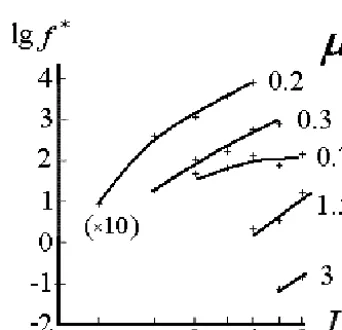
Figure 1.Functionsf∗(L) for protons with differentµ(from 0.3 to 7 keV nT−1) calculated with ISEE-1 data from Williams and Frank (1984) for a slightly disturbed (Kp≤2) period 17 November 1977. Hereµis given in kiloelectronvolt per nanotesla. The value off∗(s3cm−6)is 1.836×1030f.
Figure 2.Functionsf∗(L) for protons with differentµ(from 0.2 to 3 keV nT−1)calculated with Explorer-45 data from Fritz and Sp-jeldvik (1981) for the quiet period of 1–15 June 1972. Hereµis given in kiloelectronvolt per nanotesla. The value off∗(s3cm−6) is 1.836×1030f. The curve forµ=0.2 keV nT−1is raised above the other curves by 1 order of magnitude.
UT). The measurements were carried out near the noon sec-tor, in the following eight energy channels: 24–45.5–65.3– 95.5–142–210–333–849–2081 keV.
For calculating the functions f∗(µ,L), it is necessary to have the differential fluxes of particles (see Eq. 2). As a rule, to find these fluxes the count rate of particles in each channel is divided by the geometric factor of the instru-ment and by the width of the corresponding channel. The values thus obtained refer to the midpoints of the channels, i.e., to the arithmetic mean values of the energy channels,
¯
E=(E1+E2) /2, whereE1andE2are the lower and upper
bounds of this channel. But this is true only for a flat spec-trum or for the linear specspec-trum, i.e.,j (E)∝E. Sometimes the energy of the particles in the channel is defined as the geometric mean,E¯=
√
E1E2, but this is true only for the
power spectrumj (E)∝E−2. For a more accurate binding of the experimental data to a specific energy of the particles (within each channel of the spectrometer) and calculations of the functionsf∗(µ,L), I have developed a special method based on successive approximations to the integrating fluxes within the energy channels of the device. This method is de-scribed in detail in Kovtyukh (2016).
Using the ISEE-1 data of Williams and Frank (1984) for the period 17:52–21:05 UT 17 November 1977, I have calcu-lated thef∗(µ,L) for protons withµfrom 0.3 to 7 keV nT−1 by this method and constructed a radial dependences of
f∗(µ,L), which are shown in Fig. 1. The crosses in Fig. 1 show our calculated points between which the interpolation was performed by the method of least squares.
I have also made the same calculations of the functions
f∗(µ, L) for protons with α0=90◦ for Explorer-45 data,
averaged in Fritz and Spjeldvik (1981) over 60 orbits for the quiet period 1–15 June 1972. The measurements of proton fluxes on this satellite were carried out atL< 5.25 in the nine energy channels: 78.6–138.5–195.5–300 keV and 363.5–375–390–430–533–674–872 keV. The results of our calculations of the functions f∗(µ, L) for these data are shown in Fig. 2. To avoid overlapping, the curve for
µ=0.2 keV nT−1is raised above the other curves by 1 order of magnitude. As in Fig. 1, crosses in Fig. 2 show our calcu-lated points between which the interpolation was performed by the method of least squares.
In overlapping ranges of L and at the same µ the re-sults of calculations of the functionsf∗(µ,L) for the pro-ton belt, shown in Figs. 1 and 2, are in good agreement with each other, both in shape and in absolute values. A significant difference is obtained only in a narrow interval, at 0.7≤µ≤1 keV nT−1 on 3≤L≤4, where according to Explorer-45, we have flatter spectra and a radial dependence off∗. The discrepancy can apparently be related to the solar-cyclic variations of the belts, with some geomagnetic activity in November 1977, and to the difference in the averaging of the data of Explorer-45 and ISEE-1.
Positive radial gradients of the functions f∗(µ, L) in Figs. 1 and 2 show that the trapped protons diffuse mainly to the Earth.
2.2 The calculation of the rates of ionization losses of the trapped protons
Eq. (1) can be represented as follows:
∂ ∂L
D
LL
L2 ∂f∗
∂L
= f
∗
[image:4.612.82.253.328.493.2]Figure 3.The radial dependence of the rates of the ionization losses of protons with variousµcalculated with regard to the shape of the energy spectra of protons based on the ISEE-1 data from Williams and Frank (1984) for a period of 17 November 1977. Hereµ is given in kiloelectronvolt per nanotesla. The jump on these curves atL=5.0–5.5 corresponds to a sharp drop in electron density near the plasmapause. The vertical cuts on these curves markL, at which rate the Coulomb loss is equal to the charge exchange rate of the protons.
where
τ−1(µ, L)= − 1
f∗
∂f∗
∂t
cc
+ ∂f∗
∂t
ce
= −∂lnf
∗
∂t .
Without updating the belts by the radial diffusion,f∗(µ,L) decays exponentially with time constantτ (µ, L). I calculate the ionization losses of the protons (Coulomb losses and the losses to charge exchange) on the basis of experimental cross section of charge exchange presented in Claflin (1970) and Lindsay and Stebbings (2005) and on the real experimen-tal spectra of protons (for the same data of the ISEE-1 and Explorer-45).
Coulomb losses and the losses to charge exchange were calculated for the protons with specific values ofµ, and then these losses were summed. As a result, I found L depen-dences of the rates of ionization losses for the protons with different values ofµ(from 0.2 to 7 keV nT−1). For these cal-culations, I used the modern empirical models of the plas-masphere (Østgaard et al., 2003; Zoennchen et al., 2013) and exosphere (Moldwin et al., 2002; Ozhogin et al., 2012). The methodology of these calculations is described in detail in Kovtyukh (2016).
[image:5.612.323.536.68.295.2]The radial dependences of the rates of the ionization losses of the trapped protons were calculated for 17 November 1977 are shown in Fig. 3. Coulomb losses of protons calculated with regard to the functions f∗(µ, L) for this period (see Fig. 1). They correspond to ISEE-1 data. The dotted plots of these curves result from the extrapolation of the ISEE-1 data
Figure 4.The same as in Fig. 3 for the Explorer-45 data from Fritz and Spjeldvik (1981) for the period of 1–15 June 1972. Hereµis given in kiloelectronvolt per nanotesla.
on lowL. For protons withµ≥1.5 keV nT−1, the jump on these curves atL=5.0–5.5 reflects a sharp drop in electron density and, as a result, the drop in the rate of the Coulomb losses of protons near the plasmapause.
The vertical cuts on these curves mark L, at which rate the Coulomb loss is equal to the charge exchange rate of the protons; i.e., it is the boundary between the small L
area dominated by Coulomb losses and the larger L area dominated by the charge exchange loss of protons. The po-sition of this boundary (Lb)depends onµ of the protons: Lb ≈4.71×µ0.32, whereµis given in kiloelectronvolt per
nanotesla (Kovtyukh, 2016). This means thatEb≈300 keV
and that protons withE< 300 keV dominate the charge ex-change with atoms and protons withE> 300 keV dominate the Coulomb losses. AtL∼3–10 this boundary is almost in-dependent of the proton energy. This is mainly due to the fact that the ratio of the density of the electrons of cold plasma to the density of hydrogen atoms does not change very much with changing L (with the exception of the region of the plasmapause).
Figure 4 shows the radial dependence of the rates of ion-ization losses of the trapped protons calculated for the quiet period 1–15 June 1972. Coulomb losses of protons are cal-culated with regard to the functions f∗(µ, L) for this pe-riod (see Fig. 2). They correspond to Explorer-45 data. From these data, in the region dominated by the Coulomb losses of protons, atL< 4, the spectra of protons were flatter than the spectra measured on ISEE-1 for the period 17 November 1977, and therefore the losses of protons were less. On an-other hand, Explorer-45 data, compared to ISEE-1 data, were obtained in a period of higher solar activity; in this period the density of the plasmasphere and exosphere was apparently somewhat higher and, therefore the losses of protons, espe-cially the Coulomb losses at L< 5, was significantly more (this effect was not considered in our calculations).
In the region of the plasmapause, methodical errors of our calculations of the rates of the Coulomb losses of the trapped protons can be more than in the other regions of the belts. However, from further consideration it will be seen that this circumstance can have an effect only on the calculations of
DLL on 5≤L≤6 for protons withµ∼1.5 keV nT−1. For
protons withµ< 1.5 keV nT−1, the charge exchange is dom-inated in the region of the plasmapause, and for protons with
µ> 1.5 keV nT−1, reliable calculations of DLLcan be done
only forL> 6 (for the ISEE-1 data).
2.3 The calculation of rates of the radial transport of the trapped protons
We divide the radial dependences of f∗(µ, L) shown in Figs. 1 and 2 into separate segments and integrate Eq. (4) within each such segment taking into account Figs. 3 and 4. As a result, for each value ofµin Figs. 1 and 2, we obtain the following chain of integrodifferential equations:
DLL(µ, Li+1)
L2i+1
∂f∗ ∂L
Li+1 −
DLL(µ, Li)
L2i
∂f∗ ∂L
Li
=
Li+1
Z
Li
f∗(µ, L)
L2τ (µ, L)dL, (5)
whereLi andLi+1(i=1, 2, . . . ,n) are the lower and upper
boundaries of the corresponding segment of the radial profile
f∗(µ,L). After calculating all the derivatives and integrals in Eq. (5), we obtain a system of the linear algebraic equations for a givenµ.
The values of the two terms on the left part of Eq. (5) are very close to each other and their difference strongly depends on the radial dependence ofDLL. In addition, the system of
Eq. (5) is incomplete: the number of unknownsDLL(µ, Li)
is one more than the number of equations. It can be solved only if we exclude one of these unknowns in each system of equations (for each given value ofµ).
By summing these equations, we exclude from the system of Eq. (5) all intermediate terms, and we get the complete
equation. The difference between the normalized diffusion flows on the biggestLand on the smallestLis on the left side of this is, and the normalized integral of the rates of losses of the protons between these extremeL(for a givenµ)is on the right-hand side.
For general physical reasons, it follows thatDLLrapidly
decreases with decreasingL. This fact is reflected in all the proposed mechanisms of the radial diffusion of particles in the Earth’s radiation belts and in the belts of other planets (see, e.g., Kollmann et al., 2011). Primarily, this is due to the fact that the magnetic field increases rapidly with decreasing
L.
Therefore, the diffusion flow for the smallestL is much less than for the largestL, and we can leave the flow for the largestLon the left side of the complete equation. As a result we obtain a linear equation with one unknown variable and we find from it the valueDLLat the external boundary of the
Lrange (for a givenµ). Substituting this valueDLLin
sys-tem of Eq. (5), we obtain the complete syssys-tem of equations and gradually find all the other values of DLL at different
L(for a givenµ). Similarly, one can create and resolve the system Eq. (5) for other values ofµ. However, I do not want to make any preliminary assumptions about the radial depen-dence ofDLL.
For all values ofµandL, shown in Figs. 1 and 2, I calcu-lated L−2(∂f∗/∂L)from the left part of Eq. (5). According to our calculations, for protons withµ≥1.5 keV nT−1from ISEE-1 data (Fig. 1), the valueL−2(∂f∗/∂L)monotonically decreases with decreasing L: 10.4 times when reducing L
from 10 to 4 forµ=1.5 keV nT−1, 27.3 times when reduc-ingLfrom 10 to 5 forµ=3 keV nT−1, 40.2 times when re-ducingL from 10 to 5 forµ=5 keV nT−1, and 45.4 times when reducingLfrom 10 to 6 forµ=7 keV nT−1.
So even if we assume thatDLLdoes not depend onL, the
smaller of the two terms in the left part of the total equa-tions of systems (5), for smallest L, can be neglected for protons with µ≥ 1.5 keV nT−1. The error of the calcula-tions ofDLLatL=10, related to this, ranges from∼10 %
for µ=1.5 keV nT−1 to ∼2 % for µ=7 keV nT−1 (if we posit thatDLLdecreases with decreasingL, this error will be
much less). Of course, when approaching the lower boundary onL(for a given value ofµ), the error of our calculations of
DLLincreased. To this error we must add the errors of
calcu-lationsf∗(Figs. 1 and 2) and the ionization losses of protons (Figs. 3 and 4).
However, for protons with µ=1 keV nT−1, the value
L−2(∂f∗/∂L) is reduced only 2.9 times when L is re-duced from 9 to 3. In this case, my method is valid only under the assumption that DLL quite strongly decreases
times withLdecreasing from 4.5 to 2. However, atL> 5 for
µ=0.7 keV nT−1 and atL> 4.5 for µ=0.3 keV nT−1, the value of L−2(∂f∗/∂L)increases with decreasingL.
Thus, for protons withµ< 1 keV nT−1, our calculations of
DLLaccording to ISEE-1 data are less reliable than
calcula-tions for protons withµ≥1.5 keV nT−1.
For protons with µ< 1.5 keV nT−1, the ISEE-1 data are well complemented by Explorer-45 data obtained at smaller
L. According to the Explorer-45 data (Fig. 2), the value of
L−2(∂f∗/∂L) monotonically decreases with decreasing L
for protons with µ=0.2–3 keV nT−1: 54.4 times when re-ducingLfrom 4 to 2 forµ=0.2 keV nT−1, 8.6 times when reducingLfrom 4.5 to 2.5 forµ=0.3 keV nT−1, 1.6 times when reducingLfrom 4 to 3 forµ=0.7 keV nT−1, 4.5 times when reducingLfrom 5 to 4 forµ=1.5 keV nT−1, and 1.6 times when reducing L from 5 to 4.5 forµ=3 keV nT−1. Therefore, this method appears to be applicable to Explorer-45 data for protons withµ=0.2–0.7 keV nT−1.
In calculating the derivatives on the left-hand side and in-tegrals on the right-hand side of Eq. (5), I divided the scale of
Linto fairly short intervals where the functionsf∗(µ,L) and
τ (µ, L)are well approximated by a power law with different exponents. All the approximation functions were joined to-gether at the boundaries of these intervals.
The results of our calculations of DLL(µ, L) based on
Figs. 1 and 3 (ISEE-1) are shown in Fig. 5, and those based on Figs. 2 and 4 (Explorer-45) are shown in Fig. 6. The num-bers on the right-hand side of Figs. 5 and 6 refer to the values ofµ(in kiloelectronvolt per nanotesla).
From Figs. 5 and 6, we see that the results of our cal-culations of DLL(µ, L) based on the data from ISEE-1
and Explorer-45 are in good agreement with each other for
µ=0.3 keV nT−1(they differ by no more than∼2.5 times their value). For protons with µ=0.7 keV nT−1, the func-tions ofDLL(L)are sewn together well atL=4. For protons
with 0.7 <µ< 1 keV nT−1in the region 3≤L≤4, where ac-cording to ISEE-1 and Explorer-45 (see Figs. 1 and 2) the ra-dial gradients of the functionsf∗(µ,L) are significantly dif-ferent, good agreement was also obtained between the calcu-lated values ofDLL(µ, L). However, forµ=1.5 keV nT−1
the values ofDLLcalculated atL=4.5–5.0 on the basis of
the Explorer-45 data were∼7–8 times smaller than the val-ues calculated with the ISEE-1 data.
This discrepancy is reduced if we consider that the data from Explorer-45 are obtained in a period of higher solar activity. In this period the density of the plasmasphere and exosphere was apparently higher than during the period of measurements on ISEE-1. Therefore, the losses of protons were greater than our calculated values, especially atL< 5. In this regard, the values ofDLLshown in Fig. 6 should be
increased (see Eqs. 4 and 5).
The errors of my method of calculating DLL depend on
[image:7.612.324.527.67.229.2]the width of the range ofLin which we have conducted the calculations: the narrower this range, the more errors there are in our calculations. For differentµthe width of the range
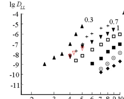
Figure 5.The results of calculations of the values ofDLL(µ, L)
near the equatorial plane based on the ISEE-1 data in Williams and Frank (1984) for the weakly disturbed period from 17:52 to 21:05 UT, 17 November 1977. In this period Kp=1− (Kp≤2+
for 12 h prior to this period UT). These results take into ac-count Figs. 1 and 3. Red signs show values of DLL for
pro-tons with µ=1 keV nT−1, calculated according to ISEE-1 data in Williams (1981) for the quiet period of 24–25 November 1977 (Kp≤1). Here,DLLis given in values per second andµis given in
kiloelectronvolt per nanotesla.
Lis different. For sufficiently long series of calculations (for large numbers of Eq. 5), when the maximum (at the upper limit of the rangeL) and the minimum (at the lower end of this range) values ofDLLdiffer by more than 1 order of
mag-nitude, i.e., forµfrom 0.3 to 5 keV nT−1based on the ISEE-1 data and forµ∼0.2 keV nT−1 based on the Explorer-45 data, errors of our calculations ofDLLdo not exceed 10 % at
largeL. With decreasingLand with increasingµof protons, these errors increase to some tens of percent.
Since the Explorer-45 data are limited to a maximum availableL∼5, correct calculations ofDLLfrom these data
are possible only forµ< 1 keV nT−1. For large values ofµ
the ranks of our calculations ofDLLon the scale ofL are
short, which leads to large methodical errors and to a signif-icant underestimation ofDLLin the calculations for protons
withµ> 1 keV nT−1based on the Explorer-45 data.
ForL> 5 the magnetosphere is asymmetric in magnetic local time (MLT), and with the growth ofLthis asymmetry increases. Because in the quiet periods the asymmetry of the magnetosphere for 5 <L< 10 is not very large and the func-tionf (µ,L) in Eq. (1) as the functionf∗(µ,L) in Eq. (5) is averaged over the drift of particles around the Earth, the average values ofLare close to the values given in Fig. 5. According to our estimates, the associated error does not ex-ceed other methodical errors in our calculations.
The transition from a dipole model to a more realistic mathematical model of the geomagnetic field leads to some changes in the calculated values of DLL(µ, L). However,
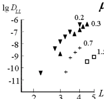
Figure 6.The results of calculations of the values ofDLL(µ, L)
near the equatorial plane based on the averaged Explorer-45 data in Fritz and Spjeldvik (1981) for the quiet period of 1–15 June 1972. These results take into account Figs. 2 and 4. HereDLLis given in
values per second andµis given in kiloelectronvolt per nanotesla.
slightly disturbed (Kp < 2) periods. The ISEE-1 data relate to near-noon sector of MLT, and the Explorer-45 data were obtained atL< 5. So, we can hope that the deviations of the geomagnetic field from the dipole configuration in the outer regions of the trap will not lead to significant changes in the calculated values of DLL(µ, L), and our main conclusions
will not change.
Taking into account all possible errors, the calculated val-ues ofDLL(µ, L)are shown in Figs. 5 and 6. These deviate
from the real values by no more than∼2.5 times their own value and, as a rule, do not exceed the size of the symbols in Figs. 5 and 6 (for all values ofLandµof protons considered here, except forµ=1.5 keV nT−1in Fig. 6).
This is confirmed by a comparison between our cal-culations according to data from ISEE-1 for the period 17 November 1977 and according to those from 24–25 November 1977. For these periods, we obtained values of
DLL(µ, L)that were close to each other at the same values of
µandL. For protons with 0.5≤µ≤3 keV nT−1, they differ by no more than 1.5–2.0 times their own value. For compar-ison, red signs in Fig. 5 show several values ofDLLfor
pro-tons with µ=1 keV nT−1, calculated according to ISEE-1 data (Williams, 1981) for the quiet period of 24–25 Novem-ber 1977 (Kp≤1).
In the total errors of our calculations of DLL, the errors
associated with models of the plasmasphere (see Kovtyukh, 2016) play a major role. To this rather large value (up to∼2.5 times) much smaller errors of the measurements of proton fluxes based on ISEE-1 and Explor45 and methodical er-rors (see above) are added. Some erer-rors can also be added by physical processes unaccounted for here, such as plasma in-stability and the interaction of protons with electromagnetic waves and micro-injections of hot plasma from the tail of the magnetosphere (for low-energy protons at large L).
How-ever, our calculations are carried out for quiet and weakly disturbed periods in Earth’s magnetosphere when the plasma distribution is stable, and fast dynamic processes can be ne-glected in comparison with radial diffusion.
3 Discussion
It has been shown that atL> 3, all stationary distributions (spatial, energy and pitch angle) of protons (and other ions) of the Earth’s radiation belts are interrelated and should be formed by mechanisms which provide the radial trans-port of these particles while conservingµandK. Kovtyukh (1984, 1985a, b, 1989, 1994, 1999a, b, 2001) has given the fullest and most comprehensive justification of this in-terrelation in the distributions of protons (and other ions) as a result of the data analysis of 22 missions (Explorer-12, Explorer-14, Mariner-4, Explorer-33, European Space Research Organisation satellite 2 (ESRO-2), 4, Injun-5, 1968-26B, Orbiting Vehicle 1-19 (OV1-19) , Explorer-45, 1972-076B, Molnija-1, Applications Technology Satel-lite 6 (ATS-6), Molnija-2, ISEE-1, Spacecraft Charging at High Altitudes (SCATHA), AMPTE/Charge Composition Explorer (CCE), 21, Akebono, CRRES, Gorizont-35 and the Engineering Test Satellite VI (ETS-VI)) for 34 years of space research (1961–1994). For protons with
µ> 0.5±0.2 keV nT−1, such a situation can only be pro-vided by mechanisms of the radial diffusion of particles to the Earth from the outer boundary of belts while conserving
µandK(Kovtyukh, 2001).
The main result of our calculations is the strong depen-dence ofDLLnot only onLbut also onµ. Figures 5 and 6
show that for all consideredL, the values ofDLL decrease
rapidly with increasing values ofµ.
This result can be seen from Figs. 1–4 and Eq. (4) before
DLL(µ, L)is calculated: for any given L, the rates of the
ionization losses of protons decrease with increasingµ(see Figs. 3 and 4), but the value(∂lnf∗/∂L) increases or re-mains almost unchanged (see Figs. 1 and 2). Therefore, to keep the balance of radial diffusion and loss of particles, the coefficient ofDLL should decrease with µ increasing.
If other possible losses (primarily, the interaction of protons with the waves) are take into account, the dependence ofDLL
onµonly increases.
The effect of reducingDLLwith increasingµis clearly
ex-pressed in the ISEE-1 data presented in Fig. 2a in Williams (1981). From this figure, it is seen that the radial gradient off (µ,L) increases sharply in the transition from high to low L. The greater µ is, the more L there is, where this happens. This effect indicates a decrease inDLLwithµ
The mechanism of particle transport under the influence of SI was proposed by Kellogg (1959), and in many works it has been used as the main mechanism. It is implemented when fluctuations in the dynamic pressure of the solar wind influ-ence the magnetosphere and is usually called magnetic dif-fusion. I denote the diffusion coefficient for this mechanism byDLLM . Models of the Earth’s radiation belts based on the mechanism of magnetic diffusion were created by Nakada and Mead (1965) and Tverskoy (1965, 1969). In the model of Nakada and Mead (1965),DMLL=2.3×10⁻¹⁵×L10s−1. In the model of Tverskoy (1965, 1969),DLLM =5×10⁻¹⁴×
L10s−1. In these models it is supposed that the spectrum of magnetic fluctuations has a power-law form with an expo-nent of−2; in this caseDMLL does not depend on the drift frequency of the particles or their energy andµbut only on
L.
The mechanism of magnetic diffusion is efficient only for traps with a strong azimuthal asymmetry of the geomagnetic field. But in the depths of the geomagnetic trap the magnetic field is almost symmetric and, therefore, the efficiency of the magnetic diffusion should be very small.
Another popular mechanism of radial transport of trapped particles is their diffusion under the action of the fluctuations of an electric field in the magnetosphere during substorms (Fälthammar, 1965, 1966, 1968; Cornwall, 1968, 1972). In contrast to the vortex electric fields generated in the magne-tosphere during SI, the electric field of a substorm can be described with an electric potential, and such a mechanism of particle transport is usually called electric diffusion. It does not depend on the azimuthal asymmetry of the mag-netic field. In this mechanism DLL depends on µ and on
the charge of the particles. I denote the diffusion coefficient for this mechanism by DELL. According to Cornwall (1968, 1972), for protons
DLLE =(1.5×10⁻¹⁰−1.5×10⁻⁹) L 10
L4+µ2, (6)
whereDLLE is measured as values per second andµis mea-sured in megaelectronvolt per gauss. For µ> 5 keV nT−1 (> 500 MeV G−1) at L> 5,µ2L4 and, according to Eq. (6),DLLE ∝µ−2L10, but for lower values of µ, the de-pendence ofDELLonLis weakened at largeL.
Equation (6) for DLLE and the expression for DMLL were parameterized for Kp by Brautigam and Albert (2000). With Kp=1 the expression for DELL in Brautigam and Albert (2000) corresponds to Eq. (6) with the coefficient on the right-hand side of the expression ∼9×10⁻¹⁰, and
DLLM ∼1.8×10⁻¹⁴×L10s−1; i.e., they correspond to the average ofDLLM given by Nakada and Mead (1965) and Tver-skoy (1969). According to Brautigam and Albert (2000), with Kp increasing from 1 to 6, the values ofDLLE increase ∼200 times and the values ofDMLLincrease∼340 times.
The functions of DLLM andDLLE depend onL andµ in different ways, and therefore in different regions of {L,µ},
space their ratio is different. AsDELLdepends onµand de-creases with decreasingL to less thanDLLM, if DMLL domi-nates at largeL,DLLE can dominate at smallL. IfDELL domi-nates for smallµ,DLLM can dominate for largeµ. In addition, this ratio can change depending on magnetic activity.
These circumstances lead to different conclusions for the ratio ofDMLLtoDELL. The conclusions were drawn in differ-ent articles and are sometimes incompatible with each other. So, for electrons withµ=5–50 keV nT−1and related fluc-tuations of the electric field atL=3–7, it has been argued based on CRRES data thatDLLE DMLL(Brautigam et al., 2005), but based on the fluctuations of the magnetic field at ground stations and based on AMPTE and GOES data, it has been argued, for the sameLand for the sameµof elec-trons, thatDLLM DLLE (Ozeke et al., 2012) for both Kp=1 and Kp=6 (see Fig. 11 in Ozeke et al., 2012). In Ozeke et al. (2014), the conclusions of Ozeke et al. (2012) were sup-ported by the analysis of data from CRRES and GOES, and another parameterization, different from that of Brautigam and Albert (2000), was proposed forDELLandDLLM for Kp (andL) where these parameters do not depend onµ.
In many works,DLLM andDLLE have been considered to be modes of radial diffusion that are independent of each other. In our calculations ofDLL, I only used data for the
parti-cles and did not carry out a separation ofDLLfor different
modes. In the course of further discussion it will be shown that the function ofDLL(µ, L)calculated here corresponds
to the uniform diffusion mode which operates in a broad band onLand the energies of protons.
The values ofDLLare determined by the spectral density
of the fluctuations (pulsations) of the electric and magnetic fields (Schulz and Lanzerotti, 1974). In theoretical works a power dependence of DLL on L is usually postulated:
DLL∝Ln. This corresponds to the power spectra of the
fluc-tuations of the fields. For different mechanisms of the radial diffusion of the particles, the parameterntakes different val-ues. Therefore, in sufficiently wide ranges ofL, the depen-dence ofDLL onL for particles with a fixedµ is not
de-scribed by a simple power law. This is evident in the evalua-tion of the parametern, obtained from the experimental data: the parameterntakes significantly different values in differ-ent intervals ofLandµ(e.g., Schulz and Lanzerotti, 1974). According to Fig. 5, in the range ofµ∼1–7 keV nT−1, val-ues of the parametern∼7.5, 7.4, 8.2, 10 and 7.7 forµ∼1, 1.5, 3, 5 and 7 keV nT−1(averagen∼8.2).
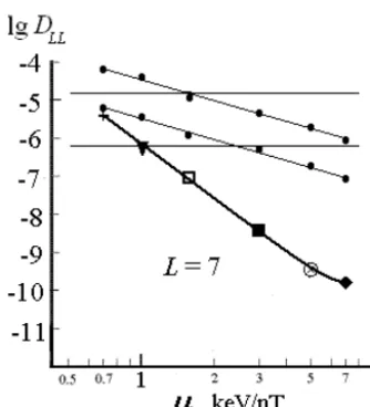
Figure 7 presents the dependence of DLL(µ) on L=7
based on the results shown in Fig. 5. HereDLLis given in
values per second andµis given in kiloelectronvolt per nan-otesla. This dependence is shown by a thick curve, and the signs on it correspond to the signs in Fig. 5. In addition, in Fig. 7 thin lines with dots show the dependences ofDLL(µ)
Figure 7.The dependence of theDLLonµforL=7. The thick
curve corresponds to the results given in Fig. 5. The thin curves correspond to Eq. (6) for the electric diffusion. The lower horizontal line is the value ofDLLin Nakada and Mead (1965), and the upper
line is the value ofDLLin Tverskoy (1965, 1969). HereDLLis
given in values per second.
magnetic diffusion, as given in Nakada and Mead (1965) and Tverskoy (1965, 1969).
Figure 7 shows that the results of our calculations are not consistent, not only with magnetic diffusion but also with electric diffusion, as described by Eq. (6). Different linear combinations of DMLL and DLLE do not lead to reasonable agreement between these results and our calculations.
Figure 8 presents the dependences ofDLL(µ)on different
L, in the range from 4 to 10, based on the results shown in Fig. 5. Here, as in Fig. 7,DLLis given in values per second
and µis given in kiloelectronvolt per nanotesla. The thick lines in this figure are calculated using the method of least squares. The numbers near these lines correspond to the val-ues ofL.
According to Fig. 8,DLL(µ)∝µ−m, where the parameter
m depends on L. The maximum value of m(∼4.4–4.5) is achieved atL∼6–7; the minimumm(∼2.4) is achieved at
L=4. The value of this parameter averaged overL equals 3.9 (or 4.1 if excluding the value ofmforL=4).
The results of our calculations of DLL, shown in
Figs. 5 and 8, for protons withµfrom∼0.7 to∼7 keV nT−1 atL≈4.5–10, are most adequately described by the follow-ing expressions:
DLL(µ, L)≈4.9×10⁻¹⁴µ−4.1L8.2, (7)
whereDLLis measured in values per second andµis
mea-sured in kiloelectronvolt per nanotesla. ReplacingµbyEin Eq. (7), we get
[image:10.612.311.542.66.244.2]DLL(E, L)≈1.3×10⁵(EL)−4.1, (8)
Figure 8.The dependences ofDLL(µ)on differentL(in the range
from 4 to 10), which corresponds to the results shown in Fig. 5. HereDLLis given in values per second.
whereDLLis measured in values per second andEis
mea-sured in kiloelectronvolt. ReplacingELby drift frequency in Eq. (8), we get
DLL(fd)≈1.2×10⁻⁹fd−4.1, (9)
wherefd is the azimuthal drift frequency of nonrelativistic protons (inverse value of the drift period of a particle around the Earth),fdis measured in millihertz andDLLis measured
in values per second.
In Eqs. (7)–(9) the results of the calculations ofDLL for
protons withµ=0.3 keV nT−1 are not taken into account. These differ greatly (see Fig. 5) from the results of the calcu-lations for protons withµ≥0.7 keV nT−1. They correspond to the low-energy part of the spectra of protons, and even in quiet periods, this part of the spectra of trapped particles is very sensitive to the cyclotron and other plasma instabilities that were not taken into account in our calculations.
The Eqs. (7)–(9) contradict the theory of diffusion under the action of SI (magnetic diffusion). According to this the-ory,DLL does not depend on theµ,E andfd of particles
(Nakada and Mead, 1965; Tverskoy, 1965, 1969; Schulz and Lanzerotti, 1974).
In the dipole approximation, the azimuthal drift frequency of nonrelativistic trapped particles is fd=11.8×µ L−2, wherefdis given in millihertz and µis given in kiloelec-tronvolt per nanotesla. The results for protons withµ=0.3, 0.7, 1, 1.5, 3, 5 and 7 keV nT−1shown in Fig. 5 correspond to
fd∼0.14–0.57, 0.13–0.52, 0.15–0.74, 0.18–0.87, 0.35–0.98,
0.59–1.20 and 0.83–1.68 mHz. These frequencies belong to the range of Pc6.
For magnetic field fluctuations DLL∝ fd2PM(fd)L10
(Fälthammar, 1965; Nakada and Mead, 1965; Tverskoy, 1965), and for electric field fluctuationsDLL ∝PE(fd)L6
spectral density of these fluctuations (pulsations). Therefore, to satisfy the Eqs. (7)–(9), the spectrum of magnetic field fluctuations should have an exponent of about−6 and should be attenuated with increasing L as L−10. The spectrum of electric field fluctuations should have an exponent of about −4 and should be attenuated with increasingLasL−6.
Unfortunately, in the range of f< 1 mHz the spectra of fluctuations (pulsations) of the electric and magnetic fields in the geomagnetosphere and in the surrounding area are insuf-ficiently studied. In the range of 0.1–1.7 mHz (Pc6) spectra of these fluctuations are irregular and vary strongly. Compared to higher-frequency ranges, there were few reliable measure-ments of the pulsations of the electric and magnetic fields in this interval until the recent publication of the results from experiments on THEMIS.
According to the measurements of the Geotail and Wind satellites in the near-Earth foreshock (Berdichevsky et al., 1999), typical spectra of the magnetic field fluctuations in the range of∼0.5–100 mHz can be approximated by a power law with an exponent of−4 to−2. In the upper part of this range (> 10 mHz), some of these spectra can be approximated by a power law with an exponent of−6, but at the bottom of the range (< 10 mHz) the spectrum is flatter and the exponent is close to the value−2 (see Fig. 8 in this article). This is confirmed by CRRES data (Ali et al., 2015): in the range of ∼1–8 mHz averaged spectra of the magnetic field fluctua-tions are very hard and almost flat.
In the range of 1–100 mHz the spectra of the fluctuations of the magnetic field were also measured at ground stations associated with cusp/cleft (Posch et al., 1999). These spectra are irregular and vary strongly depending on the speed of the solar wind. For a power-law approximation, the average ex-ponent of these spectra is close to the value−4 in the range of 10–100 mHz, but in the lower part of the range (1–10 mHz) an exponent of the spectral density of these fluctuations is close to−5/3 (see Fig. 6 in this article).
According to GOES (on geosynchronous orbit) and Wind (in the solar wind) in the range of 0.2–1.7 mHz (Kepko and Spence, 2003), the amplitude spectra of magnetic fluctua-tions are irregular (fine structure with narrow peaks), but the average amplitude of these fluctuations decreases with in-creasing frequency by a power law with an exponent of−1.8 to−1.5 (see Figs. 4, 9, 11, 13 and 15 in this article); i.e., for the average spectral density we have an exponent of−4.6 to −4.0.
Thus, the experimental spectra of the magnetic field fluc-tuations (pulsations) are not consistent with Eqs. (7)–(9) ob-tained here.
On the basis of over 7 years of averaged data from THEMIS for all MLT, for different Kp (from 0 to 5) and for differentL(from 3.5 to 7.5), Liu et al. (2016) constructed the spectra of electric field fluctuations (pulsations) in the range of ∼0.5–10 mHz (unfortunately, the data at f< 0.5 mHz are not given). In the range of ∼0.5–2 mHz these spectra are very soft, especially during quiet and slightly disturbed
(Kp=0–2) periods. For Kp=0–2, according to Fig. 2 from Liu et al. (2016), in the range of∼0.5–2 mHz the depen-dence of the spectral density of the fluctuations on the fre-quency can be approximated by a power law with an expo-nent that varies from−(3.3–3.9) atL> 5.5 to−5.4 atL=4.5 and−10.5 atL=3.5; i.e., at L≥4.5 the average value of this exponent is close to−4. Our calculations also show that the slope of the radial dependence ofDLL(µ, L)usually
in-creases with decreasingL(see Figs. 5 and 6).
According to Fig. 2 in Liu et al. (2016), at a frequency of∼0.5 mHz the spectral density of the electric field fluc-tuations decreases also with increasingL(approximately as
Lk, where mean square value of the exponentkis changed from−6.5 when Kp=0 to−7.3 when Kp=2). But already at a frequency of∼1.0 mHz this spectral density does not depend onL, and at frequencies of∼1 to 10 mHz this value increases withL.
Thus, according to THEMIS data averaged over 7 years for all MLT, for periods with Kp=0–2 the spectral den-sity of the electric field fluctuations (pulsations) atL≥4.5 for f ∼0.5–1 mHz can be described by the following ex-pression:PE∝fd−4L−6. Substituting this expression into the
formulaDLL∝PE(fd)L6(Fälthammar, 1966, 1968) for the
radial diffusion of particles influenced by the electric field fluctuations, we obtainDLL∝fd−4. This result corresponds
to our Eq. (9), and, hence, it is consistent with Eq. (8) and Eq. (7), which refer to the main cluster of calculated points in Fig. 5 and satisfy the rangesfd∼0.5–1.2 mHz (Pc6) and Kp=0–2.
On the basis of the spectra of electric field fluctua-tions, Liu et al. (2016) calculatedDLLfor relativistic
elec-trons withµ=5−40 keV nT−1 (500–4000 MeV×G−1)at
L=3.5–7.5. The drift frequency of these electrons corre-sponds to the rangefd∼1–4 mHz (Pc5), where the spectrum
of fluctuations is flatter and the spectral density increases withL. For these reasons, in comparison to our calculations for protons for a rangefd∼0.15–1.2 mHz (Pc6), in Liu et al.
(2016) the dependence ofDLLonµis much weaker and the
dependence ofDLLonLis slightly stronger.
Note that for electrons with µ=1–50 keV nT−1 in the range ofL=3–7 , the functions ofDLLare calculated also
for the spectra of electric field fluctuations in the range of 0.2–15.9 mHz measured by CRRES (Brautigam et al., 2005). For Kp=1, about the same dependence ofDLLonLis
ob-tained as in Eq. (7) (DLL∝L8), but the dependence ofDLL
onµwas much weaker (see Fig. 9 in Brautigam et al., 2005).
4 Conclusion
I calculate the valueDLL, which is a measure of the rate of
This is done by successively solving the equations of the balance of the radial transport/acceleration and ionization losses of protons for the stationary belt. Calculations of the ionization losses of protons (Coulomb losses and charge ex-change) were carried out on the basis of modern models of the plasmasphere and the exosphere.
To find DLL I calculated the radial dependences of the
distribution function f∗(L,µ)for different µ. For each of the given values of µ, these dependences were divided into short segments and the systems (chains) of integrodifferen-tial equations describing the balance of radial transport and losses of protons were solved. This work is carried out here for the first time.
For these calculations I used the data of ISEE-1 for protons with an energy of 24 to 2081 keV atL≈2–10 and the data of Explorer-45 for protons with an energy of 78.6 to 872 keV at
L≈2–5. The values ofDLLcalculated from the data of
ISEE-1 and Explorer-45, in the overlapping intervals ofLandµ, are in good agreement with each other.
As a result of the calculations, I found that in the range of
L≈2.5–10 the dependences ofDLL(L)are significantly
dif-ferent for protons with difdif-ferentµ(from 0.2 to 7 keV nT−1). The values of DLL decrease rapidly with decreasingL as
well as with increasingµ.
It is shown that for protons with µ from ∼0.7 to ∼7 keV nT−1atL≈4.5–10, the functions ofDLLcan be
ap-proximated by the following equivalent expressions:DLL≈
4.9×10⁻¹⁴µ−4.1L8.2, or DLL≈ 1.3×10⁵(EL)−4.1, or
DLL≈ 1.2×10⁻⁹fd−4.1, wherefdis the drift frequency of
the protons (in mHz),DLLis given in values per second,E
is given in kiloelectronvolt andµis given in kiloelectronvolt per nanotesla. These expressions are obtained for quiet and weakly disturbed conditions in the magnetosphere (Kp≤2). During magnetic stormsDLLincreases, and the expressions
obtained here forDLLcan change completely.
These results contradict the mechanism of the radial diffu-sion of particles under the influence of sudden impulses (SI) of the magnetic field and also under the influence of substorm impulses of the electric field, as was suggested by Conwall (1968, 1972).
It is shown that the bulk of the calculations ofDLL, in the
range of ∼0.5–1.2 mHz (Pc6), is consistent with spectra of the fluctuations (pulsations) of the electric field atL∼4.5– 7.5 during quiet and weakly disturbed periods (Kp≤2) aver-aged over 7 years for all MLT according to THEMIS data in Liu et al. (2016. These ranges offdandLcorrespond to the trapped protons with energies from∼0.18 to∼0.7 MeV and electrons with energies from∼0.21 to∼1.19 MeV.
The comparisonDLL for protons in a certain region {µ,
L} with electric field pulsations in the appropriate frequency range shows a close relationship between the radial diffusion of particles and the pulsations of the electric field. For higher frequencies (in the range of Pc5), the experimental spectra of these pulsations are flatter and the spectral density increases by about 1 order of magnitude with the increase in Lfrom
3.5 to 7.5. Therefore, for more energetic particles of the ra-diation belts corresponding to higher drift frequencies, other dependences ofDLLonµandLmay exist. This applies in
particular to the relativistic and ultra-relativistic electrons of the radiation belts.
Because the values ofDLLwere calculated here only for
two short periods (quiet and weakly disturbed) according to only two missions (ISEE-1 and Explorer-45) near the equa-torial plane and only for protons in the limited ranges ofµ
andL, they cannot of course be regarded as complete and final. This work should be continued.
Acknowledgements. The author would like to thank P. Kollmann (Applied Physics Laboratory, Johns Hopkins University) for very important and fruitful comments on and proposals regarding the paper and E. Roussos (Max Planck Institute for Solar System Re-search) for editing the paper. The author thanks the Kyoto World Data Center for Geomagnetism for providing the Dst indices.
The topical editor, E. Roussos, thanks P. Kollmann, S. Bour-darie, and one anonymous referee for help in evaluating this paper.
References
Ali, A. F., Elkington, S. R., Tu, W., Ozeke, L. G., Chan, A. A., and Friedel, R. H. W.: Magnetic field power spectra and magnetic radial diffusion coefficients using CRRES magnetometer data, J. Geophys. Res., 120, 973–995, doi:10.1002/2014JA020419, 2015.
Alinejad, N. and Armstrong, T. P.: Radial diffusion of geo-magnetically trapped protons observed by the Galileo En-ergetic Particle Detector, J. Geophys. Res., 111, A09209, doi:10.1029/2005jA011040, 2006.
Berdichevsky, D., Thejappa, G., Fitzenreiter, R. J., Lepping, R. L., Yamamoto, T., Kokubun, S., McEntire, R. W., Williams. D. J., and Lin, R. P.: Widely spaced wave-particle observations during GEOTAIL and Wind magnetic conjunctions in the Earth’s ion foreshock with near-radial interplanetary magnetic field, J. Geo-phys. Res., 104, 463–482, doi:10.1029/1998JA900018, 1999. Beutier, T., Boscher, D., and France, M.: SALAMMBO: A
three-dimensional simulation of the proton radiation belt, J. Geophys. Res., 100, 17181–17188, doi:10.1029/94JA02728, 1995. Blake, J. B., Kolasinski, W. A., Fillius, R. W., and Mullen, E. G.:
Injection of electrons and protons with energies of tens of MeV intoL< 3 on 24 March 1991, Geophys. Res. Lett., 19, 821–824, doi:10.1029/92GL00624, 1992.
Brautigam, D. H. and Albert, J. M.: Radial diffusion anal-ysis of outer radiation belt electrons during the October 9, 1990, magnetic storm, J. Geophys. Res., 105, 291–309, doi:10.1029/1999JA900344, 2000.
Brautigam, D. H., Ginet, G. P., Albert, J. M., Wygant, J. R., Row-land, D. E., Ling, A., and Bass, J.: CRRES electric field power spectra and radial diffusion coefficients, J. Geophys. Res., 110, A02214, doi:10.1029/2004JA010612, 2005.
Claflin, E. S.: Charge-exchange cross sections for hydrogen and he-lium ions incident on atomic hydrogen: 1 to 1000 keV, Rep. TR-0059(6260-20)-1, The Aerospace Corporation, El Segundo, CA, USA, 1970.
Cornwall, J. M.: Diffusion processes influenced by conjugate-point wave phenomena, Radio Sci., 3, 740–744, doi:10.1002/rds196837740, 1968.
Cornwall, J. M.: Radial diffusion of ionised helium and protons: A probe for magnetosphere dynamics, J. Geophys. Res., 77, 1756– 1770, doi:10.1029/JA077i010p01756, 1972.
Fälthammar, C.-G.: Effects of time-dependent electric fields on geo-magnetically trapped radiation, J. Geophys. Res., 70, 2503–2516, doi:10.1029/JZ070i011p02503, 1965.
Fälthammar, C.-G.: On the transport of trapped particles in the outer magnetosphere, J. Geophys. Res., 71, 1487–1491, doi:10.1029/JZ071i005p01487, 1966.
Fälthammar, C.-G.: Radial diffusion by violation of the third adia-batic invariant, in Earth’s Particles and Fields, Ed. B. M. McCor-mac, Springer, New York, USA, 157–169, 1968.
Fritz, T. A. and Spjeldvik, W. N.: Steady-state observations of geo-magnetically trapped energetic heavy ions and their implications for theory, Planet. Space Sci., 29, 1169–1193, doi:10.1016/0032-0633(81)90123-9, 1981.
Holzworth, R. H. and Mozer, F. S.: Direct evaluation of the radial diffusion coefficient near L=6 due to elec-tric field fluctuations, J. Geophys. Res., 84, 2559–2566, doi:10.1029/JA084iA06p02559, 1979.
Jentsch, V.: On the role of external and internal source in generat-ing energy and pitch angle distributions of inner-zone protons, J. Geophys. Res., 86, 701–710, doi:10.1029/JA086iA02p00701, 1981.
Kellogg, P. J.: Van Allen radiation of solar origin, Nature, 183, 1295–1297, doi:10.1038/1831295a0, 1959.
Kepko, L. and Spence, H. E.: Observations of discrete, global magnetospheric oscillations directly driven by so-lar wind density variations, J. Geophys. Res., 108, 1257, doi:10.1029/2002JA009676, 2003.
Kollmann, P., Roussos, E., Paranicas, C., Krupp, N., Jack-man, C. M., Kirsch, E., and Glassmeier K.-H.: Energetic particle phase space densities at Saturn: Cassini observa-tions and interpretaobserva-tions, J. Geophys. Res., 116, A05222, doi:10.1029/2010JA016221, 2011.
Kovtyukh, A. S.: The magnetosphere used as an analyser of spectral form of radiation belt particles, Geomagn. Aeron., 24, 566–570, 1984.
Kovtyukh, A. S.: Interrelation of radial dependence of hardness and shape of proton spectra in the Earth’s radiation belts, Geomagn. Aeron., 25, 23–28, 1985a.
Kovtyukh, A. S.: On the form of energy spectrum of protons of the Earth’s radiation belts and the mechanisms of its formation, Geomagn. Aeron., 25, 886–892, 1985b.
Kovtyukh, A. S.: Double-peak space-energy structure of the outer ion radiation belt, Geomagn. Aeron., 29, 22–26, 1989.
Kovtyukh, A. S.: The relationship between the pitch-angle and en-ergy distributions of ions in the Earth’s radiation belts, Geomagn. Aeron., 33, 453–460, 1994.
Kovtyukh, A. S.: Solar-cycle variations of invariant parameters of ion energy spectra of the Earth’s radiation belts, Cosmic Res., 37, 53–64, 1999a.
Kovtyukh, A. S.: Mechanisms of formation of invariant parameters and scaling of ion spectra in a geomagnetic trap, Cosmic Res., 37, 217–229, 1999b.
Kovtyukh, A. S.: Geocorona of hot plasma, Cosmic Res., 39, 527– 558, doi:10.1023/A:1013074126604, 2001.
Kovtyukh, A. S.: Radial dependence of ionization losses of pro-tons of the Earth’s radiation belts, Ann. Geophys., 34, 17–28, doi:10.5194/angeo-34-17-2016, 2016.
Lanzerotti, L. J. and Wolfe, A.: Particle diffusion in the geomagne-tosphere: Comparison of estimates from measurements of mag-netic and electric field fluctuations, J. Geophys. Res., 85, 2346– 2348, doi:10.1029/JA085iA05p02346, 1980.
Lanzerotti, L. J., Maclennan, C. G., and Schulz, M.: Radial diffusion of outer-zone electrons: An empirical approach to third-invariant violation, J. Geophys. Res., 75, 5351–5371, doi:10.1029/JA075i028p05351, 1970.
Lanzerotti, L. J., Webb, D. C., and Arthur, C. W.: Geomagnetic field fluctuations at synchronous orbit 2. Radial diffusion, J. Geophys. Res., 83, 3866–3870, doi:10.1029/JA083iA08p03866, 1978. Lindsay, B. G. and Stebbings, R. F.: Charge transfer cross sections
for energetic neutral atom data analysis, J. Geophys. Res., 110, A12213, doi:10.1029/2005JA011298, 2005.
Liu, W., Tu, W., Li, X., Sarris, T., Khotyaintsev, Y., Fu, H., Zhang, H., and Shi, Q.: On the calculation of electric diffusion coeffi-cient of radiation belt electrons with in situ electric field mea-surements by THEMIS, Geophys. Res. Lett., 43, 1023–1030, doi:10.1002/2015GL067398, 2016.
Lyons, L. R. and Williams, D. J.: Quantitative Aspects of Magneto-spheric Physics, D. Reidel, Norwell, MA, USA, 1984.
Ma, Q., Li, W., Thorne, R. M., Nishimura, Y., Zhang, X.-J., Reeves, G. D., Kletzing, C. A., Kurth, W. S., Hospodarsky, G. B., Hender-son, M. G., Spence, H. E., Baker, D. N., Blake, J. B., Fennell, J. F., and Angelopoulos, V.: Simulation of energy-dependent elec-tron diffusion processes in the Earth’s outer radiation belt, J. Geo-phys. Res., 121, 4217–4231, doi:10.1002/2016JA022507, 2016. Moldwin, M. B., Downward, L., Rassoul, H. K., Amin, R.,
and Anderson, R. R.: A new model of the location of the plasmapause: CRRES results, J. Geophys. Res., 107, 1339, doi:10.1029/2001jA009211, 2002.
Nakada, M. P. and Mead, G. D.: Diffusion of protons in the outer radiation belt, J. Geophys. Res., 70, 4777–4791, doi:10.1029/JZ070i019p04777, 1965.
Newkirk, L. L. and Walt, M.: Radial diffusion coefficient for electrons at 1.76 <L< 5, J. Geophys. Res., 73, 7231–7236, doi:10.1029/JA073i023p07231, 1968.
Østgaard, N., Mende, S. B., Frey, H. U., Gladstone, G. R., and Lauche, H.: Neutral hydrogen density profiles derived from geocoronal imaging, J. Geophys. Res., 108, 1300, doi:10.1029/2002jA009749, 2003.
Ozeke, L. G., Mann, I. R., Murphy, K. R., Rae, I. J., Milling, D. K., Elkington, S. R., Chan, A. A., and Singer, H. J.: ULF wave derived radiation belt radial diffusion coefficients, J. Geophys. Res., 117, A04222, doi:10.1029/2011JA017463, 2012.
Ozeke, L. G., Mann, I. R., Murphy, K. R., Rae, I. J., and Milling, D. K.: Analytic expressions for ULF wave radiation belt ra-dial diffusion coefficients, J. Geophys. Res., 119, 1587–1605, doi:10.1002/2013JA019204, 2014.
model derived from the IMAGE RPI measurements, J. Geophys. Res., 117, A06225, doi:10.1029/2011jA017330, 2012.
Panasyuk, M. I.: The ion radiation belts: Experiments and models, Effect of Space Weather on Technology Infrastructure, edited by: Daglis, I. A., Kluwer Academic Publ., the Netherlands, 65–90, 2004.
Posch, J. L., Engebretson, M. J., Weatherwax, A. T., Detrick, D. L., Highes, W. J., and Maclennan, C. G.: Characteristics of broad-band ULF magnetic pulsations at conjugate cusp latitude sta-tions, J. Geophys. Res., 104, 311–331, doi:10.1029/98JA02722, 1999.
Roederer, J. G.: Dynamics of Geomagnetically Trapped Radiation. Springer, NY, USA, 1970.
Schulz, M. and Lanzerotti, L. J.: Particle Diffusion in the Radiation Belts, Springer, NY, USA, 1974.
Selesnick, R. S., Baker, D. N., Jaynes, A. N., Li, X., Kanekal, S. G., Hudson, M. K., and Kress, B. T.: Inward diffusion and loss of radiation belt protons, J. Geophys. Res., 121, 1969–1978, doi:10.1002/2015JA022154, 2016.
Spjeldvik, W. N.: Equilibrium structure of equatorially mir-roring belt protons, J. Geophys. Res., 82, 2801–2808, doi:10.1029/JA082i019p02801, 1977.
Tomassian, A. D., Farley, T. A., and Vampola, A. L.: Inner-zone energetic-electron repopulation by radial diffusion, J. Geophys. Res., 77, 3441–3454, doi:10.1029/JA077i019p03441, 1972. Tu, W., Elkington, S. R., Li, X., Liu, W., and Bonnell, J.:
Quantify-ing radial diffusion coefficients of radiation belt electrons based on global MHD simulation and spacecraft measurements, J. Geo-phys. Res., 117, A10210, doi:10.1029/2012JA017901, 2012. Tverskoy, B. A.: Dynamics of the radiation belts of the Earth,
Geo-magn. Aeron., 3, 351–368, 1964.
Tverskoy, B. A.: Transport and acceleration of charged particles in the Earth’s magnetosphere, Geomagn. Aeron., 5, 517–530, 1965. Tverskoy, B. A.: Main mechanisms in formation of the Earth’s radiation belts, Rev. Geophys., 7, 219–232, doi:10.1029/RG007i001p00219, 1969.
Walt, M.: Introduction to Geomagnetically Trapped Radiation, Cambridge Univ. Press, NY, USA, 1994.
West, H. I., Buck, R. M., and Davidson, G. T.: The dynamics of energetic electrons in the Earth’s outer radiation belt during 1968 as observed by the Lawrence Livermore National Labora-tory’s spectrometer on Ogo 5, J. Geophys. Res., 86, 2111–2142, doi:10.1029/JA086iA04p02111, 1981.
Westphalen, H. and Spjeldvik, W. N.: On the energy depen-dence of the radial diffusion coefficient and spectra of in-ner radiation belt particles: Analytic solutions and compari-son with numerical results, J. Geophys. Res., 87, 8321–8326, doi:10.1029/JA087iA10p08321, 1982.
Williams, D. J.: Phase space variations of near equatorially mirroring ring current ions, J. Geophys. Res., 86, 189–194, doi:10.1029/JA086iA01p00189, 1981.
Williams, D. J.: Ring current and radiation belts, Rev. Geophys., 25, 570–578, doi:10.1029/RG025i003p00570, 1987.
Williams, D. J. and Frank, L. A.: Intense low-energy ion popula-tions at low equatorial altitudes, J. Geophys. Res., 89, 3903– 3911, doi:10.1029/JA089iA06p03903, 1984.