PARALLEL PERFORMANCE OF SOME MULTIGRID SOLVERS FOR THREE-DIMENSIONAL PARABOLIC EQUATIONS

PARALLEL PERFORMANCE OF SOME MULTIGRID SOLVERS

FOR THREE-DIMENSIONAL PARABOLIC EQUATIONS∗

MICHAEL HOLST†_{AND FAISAL SAIED}†

Abstract. We consider the solution of parabolic PDEs in three spatial dimensions by multigrid methods on parallel architectures. The objective is to develop high performance multigrid solvers for large scale time-dependent problems. We begin with temporal semi-discretizations with several explicit and implicit schemes, followed by a uniform spatial discretization in a 3D rectangular region. A nearly optimal time-step is then determined empirically for each of the resulting methods when applied to a given test problem, and the sequential performance of each method is then compared. We examine the effect of the step size on the convergence rates of multigrid, and present results of experiments on two parallel architectures: a four processor Cray Y-MP and a fourteen processor Alliant FX/2800. Our results demonstrate that multigrid can achieve very high parallel efficiency on coarse-grained shared memory machines, and that explicit methods are not likely to be competitive with multigrid based implicit methods on such machines.

Key Words. multigrid methods, partial differential equations, time-dependent, three-dimensional, parabolic equations, parallel algorithms, Cray Y-MP, Alliant FX/2800, shared memory architectures

1. Introduction. In this paper, we consider the solution of three-dimensional parabolic partial differential equations. The objective is to develop high performance solvers using multigrid tech-niques for large scale time-dependent problems of this type. The target machines are shared memory multiprocessors, including specifically the Alliant FX/2800 and the Cray Y-MP. We begin the paper with a discussion of explicit and implicit temporal semi-discretization schemes, and examine the elliptic problems that must be solved at each time step in the implicit schemes. Our approach to solving these shifted 3D elliptic problems is to use the multigrid method. The use of implicit time stepping schemes coupled with multigrid for solution of the resulting elliptic problems has been examined by Hackbusch, Brandt et al. in [8, 17] for 2D problems. We examine the behavior of the multigrid method for implicit time discretizations of 3D problems, and focus on the efficient parallel solution of the shifted elliptic partial differential equations arising at each time step. Issues of step size selection, multigrid initialization at each time step, and multigrid convergence rates for the shifted problems naturally arise, and we attempt to answer some of these questions.

The remainder of this paper is structured as follows. In§2, we introduce the class of problems we wish to solve. In§3, we discuss time discretization techniques, and in particular we outline the approach taken in our implementations. The elliptic problems arising in implicit time discretizations are considered in§4, and we discuss the effect of the shift introduced into the operator as a result of the time step. In §5 we review multigrid methods, and discuss the current state of research on multigrid for 3D parabolic problems. Two test problems are presented in §6: the heat equation in three spatial dimensions, and a variable coefficient problem. In§ 7, we present some experiments investigating the performance of explicit and implicit methods for the test problems on a sequential computer, and examine in more detail the effect of the shifted operator on the performance of multigrid. We present performance results for our implementations on some advanced computer architectures in§ 8, namely the Alliant FX/2800 and the Cray Y-MP. Finally, we summarize our results in§9.

2. Parabolic Problems in Three Space Dimensions. We seek the solutionu=u(x, y, z, t) of a parabolic partial differential equation of the form

ut =Lu+f in Ω⊂R3,

(1)

u(x, y, z, t) =g(x, y, z, t) on∂Ω,

u(x, y, z,0) =h(x, y, z) at timet= 0,

∗_{THIS WORK WAS SUPPORTED IN PART BY NATIONAL SCIENCE FOUNDATION GRANT NO. DMS}

89-11410 AND BY RESEARCH BOARD OF THE UNIVERSITY OF ILLINOIS GRANT NO. RES BRD IC SAIED F.

†_{NUMERICAL COMPUTING GROUP, DEPARTMENT OF COMPUTER SCIENCE, UNIVERSITY OF}

where Ω is some cuboidal region inR3. We consider operators of the formL=∇ ·(a∇) +~b· ∇+c, and in particular the case when the tensorais diagonal:

Lu= ∂ ∂x a11 ∂u ∂x + ∂ ∂y a22 ∂u ∂y + ∂ ∂z a33 ∂u ∂z +b1

∂u ∂x+b2

∂u ∂y +b3

∂u ∂z +cu, (2)

whereaii, bi,andc are functions ofx, y, z,and possiblyt.

Problems of this structure arise in numerous applications involving diffusive or thermodynamic processes. Examples include groundwater and petroleum reservoir simulation, quantum mechanics, ocean acoustics, and neutron transport.

3. Time Discretizations of Parabolic Problems. The semi-discretization of the time vari-able in the parabolic pde ut =Lu+f can be accomplished in several ways, involving the use of

explicit or implicit techniques [29, 35]. Explicit methods, in which the solution at the new time step is formed by a combination of previous time step solutions, are simple to code and under-stand, and inexpensive computationally to apply at a single time step. Examples include Forward Euler, Leapfrog, DuFort-Frankel, and Runge Kutta methods. For example, we can represent the semi-discretization using Forward Euler as:

un+1_=un

+ ∆t(Ln

un

+fn

), (3)

where ∆tis the time step from timetn to time tn+1,un is the solution,fn is the forcing function,

andLn

is the elliptic operator at timetn. The functionu n₊₁

is then the new approximate solution at timetn+1, with a discretization error ofO(∆t) for this method. Of course with explicit methods

there will be stability limit on the time step size.

To avoid the stability considerations implicit methods can be used, and the step size may be chosen purely on the basis of accuracy. They are more costly to apply, requiring the solution of linear algebraic equations at each time step (or nonlinear algebraic equations, if the elliptic operator is nonlinear). Possible choices include the Backward Euler (4) and Crank-Nicolson (5) methods:

Ln+1₋ 1

∆t

un+1₌₋ 1

∆t

un

−fn+1_,

(4)

Ln₊₁

− 2 ∆t

un₊₁

=− Ln + 2 ∆t un

− fn

+fn₊₁ . (5)

Note that by introducing the variableVn

, a recursion can be used in the Crank-Nicolson method to avoid the application of the operatorL on the right hand side:

Ln₊₁

− 2 ∆t

un₊₁

=Vn

, (6)

whereVn

is defined by:

V0₌₋

L0₊ 2

∆t

u0_{− f}0_+f1 ,

Vn=−Vn−1₋

4 ∆t

un− fn+1+fn .

4. Elliptic Problems Arising in Implicit Schemes. In each of the implicit methods dis-cussed in the previous section, an elliptic partial differential equation of the following form must be solved at each time step:

L− α

∆t

u=f. (7)

For example, with Crank-Nicolson α = 2, while α = 1 for Backward Euler. Our approach to solving this shifted 3D elliptic problem is to use the multigrid method, as was done for implicit time discretizations of parabolic problems in two space dimensions in [8, 17].

Another approach appears in [28, 32, 33, 34], where 2D parabolic problems are first discretized in space, followed by time discretization to solve the resulting system of ordinary differential equations. In particular, several explicit and implicit time discretization methods are compared in [34], involving the use of various linear solvers (including multigrid) for the linear algebraic equations arising at each time step of the implicit methods.

Our purpose is to examine and compare several semi-discretizations in time of 3D parabolic problems, study the behavior of the multigrid method for different time discretizations, and focus on the efficient parallel solution of the shifted elliptic partial differential equations arising at each time step.

4.1. Shifted Elliptic Operators. It is noted in [8] that when a semi-discretization in time is performed in the case of the 2D heat equation, the resulting shifted elliptic operators at each time step are Helmholtz operators with shift α

∆t, and the behavior of classical relaxation methods, as well

as that of the multigrid method, is analyzed in [30] for model problems of this type.

Here, we examine the effect of the time shift on the convergence behavior of multigrid for 3D elliptic operators, including Helmholtz-like operators, as well as more general variable coefficient problems.

The effect of the shift is a better conditioned problem, which will have a beneficial effect on most solution techniques. In (§7), we present numerical results demonstrating how multigrid methods benefit from the shift.

4.2. Spatial Discretization of the Elliptic Problem. We put down a uniform 3D mesh of width hon Ω, and discretize the shifted elliptic operator using centered finite difference approx-imations (the 7-point stencil). Given that the elliptic operator is the general second order linear operator in equation (2), and that we order the discrete unknowns using the natural ordering, a block tri-diagonal linear systemLhuh=fhresults. We denote the block tri-diagonal system corresponding

to a mesh-width of 2has L2hu2h=f2h, and so on.

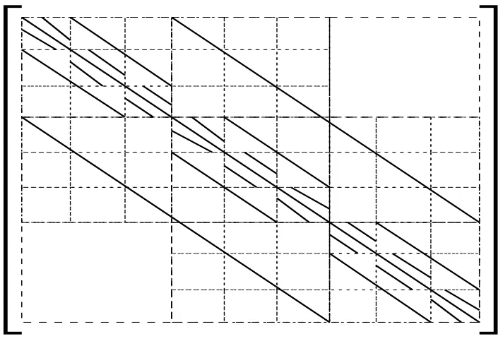
Since cross derivatives are not present in (2), the matrixLh has the non-zero structure of the

discrete 3D Laplacian (Figure 1), where the nonzeros of the matrix lie on seven diagonals. We use a data structure in our implementations that reflects the diagonal form of the discrete operator, and as a result matrix-vector operations are extremely efficient on vector computers such as the Cray Y-MP (e.g. [25]). For example, this storage format can achieve a factor of five speedup in the time taken to compute a matrix-vector product when compared to the equivalent operation implemented with more general sparse matrix storage formats, even when the gather-scatter hardware is used [27]. 5. Multigrid Methods for 3D Elliptic Problems. Multigrid methods are highly efficient techniques for solving certain types of partial differential equations. The study of these methods constitute a very active research area in numerical analysis and scientific computing, and this section represents a survey of some of the basic methods, mentioning special considerations for 3D problems. More detailed discussions can be found in any of [5, 6, 18, 30].

Fig. 1.Block tri-diagonal form of the discretized 3D elliptic operator for a3×3×3mesh.

The Two-Grid Algorithm. If uniform three dimensional meshes of widthshand 2hare used to discretize the elliptic partial differential equation discussed in § 4, we will then have two sets of equations representing discrete approximations to the original PDE; namely Lhuh = fh, and

L2hu₂h=f₂h. A two-gridCorrection Storage (CS)multigrid scheme [5, 30] using both the fine grid

and coarse grid equations to solve the underlying PDE can be represented graphically as in Figure 2 (cf. [30]).

uold h

Rν1 h

¯

uh rh=fh−Lhu¯h

I2h h

r2h

Solve

L2hc=r₂h c₂h

Ih 2h

ch ¯uh+ch

Rν2 h

unew h

Fig. 2.The two grid Correction Storage (CS) scheme.

The method begins with an initial approximation uold

h on the finest grid. A relaxation (or

smoothing) method Rh is then employed for ν₁ iterations, resulting in an approximation ¯uh with

smooth error and residual. Next, a residual computation is performed, and this residual rh is

restricted to the coarse grid via the restriction operator I2h

h , resulting in a residual on the coarse

grid,r2h.

The coarse grid problem is solved in some way (perhaps directly, or by more relaxations), and the correctionc2h obtained from the residual equation is theninterpolated back to the fine grid via

the operatorIh

2h, resulting in the correctionch. The correction is added to the approximate solution,

and ν2 smoothings are done to reduce any high frequency error that has been introduced by the

interpolation operator, resulting in the final approximationunew

h from the multigrid cycle.

Note that linearity was used to motivate the CS scheme correction equation: Le=L(u∗_{−u) =}

Lu∗_{−Lu = f −Lu = r. While there is no direct analogue in the case of a nonlinear operator}

occur in the discrete equations in particularly simple forms, which is the case in many applications such as computational fluid dynamics, then nonlinear analogues of the classical relaxation procedures such as Jacobi iteration are easily defined [7].)

A description of the two-grid Full Approximation Storage (FAS) scheme employing the more general correction scheme can be found in [5, 18]. In this scheme, a combination of the fine grid residualrh and the fine grid solution ¯uhare transferred to the coarse grid to become the right-hand

side of the coarse grid correction equation: ¯

f2h=L₂h( ¯I2 h

h u¯h) +I2 h

h (fh− Lh(¯uh)).

The correctionu2h is then returned to the fine grid as:

ch= ¯I h

2h(u2h−I2 h h u¯h).

(Note that ¯Ih2 h

1 and I h

2 h

1 may be defined independently.) While the FAS scheme is more expensive

than the CS scheme because of the more complicated formula for ¯f2h, it has several advantages: it

can be used for both linear and nonlinear problems, whereas the CS scheme is restricted to the linear case; truncation error estimates are easily obtained, enabling adaptive implementations, including adaptive time step-size control for the parabolic problems we are considering in this paper.

Smoothers. The smoothing operator Rh can be chosen to be one of the classical methods

such as Jacobi, Red/Black Gauss-Seidel (point, line, and plane versions), or weighted Jacobi. Of particular interest for 3D problems are the alternating plane relaxations, which become increasingly important for problems with anisotropic or discontinuous coefficients [9, 31]. Other methods that have been proposed include incompleteLU factorizations, as well as the conjugate gradient method [1]. The 2D multigrid method itself has been proposed as a smoother for 3D multigrid [9, 31].

The results presented in this paper are based on the weighted Jacobi method, which can be written for a linear systemAx=b as:

x(n₊₁₎

=x(n₎

+ωD−1_(b−Ax(n)_),

whereD represents the diagonal of the matrixA.

Grid Transfer Operators. The grid transfer operators we have used are the natural 3D extensions of some of the standard 2D operators, as described in [24]. In particular, we use a 3D full weighting restriction operator for fine to coarse grid transfers, which involves twenty seven fine grid points to form a single coarse grid point, and a tri-linear interpolation operator for coarse to fine grid transfers.

Solution of the Coarse Grid Problem. Our choice of the coarse grid solution technique was banded Gaussian elimination [10]. For reasons discussed in [22], we typically use enough grid levels so that the percentage of time spent in coarse grid solves amounts to roughly five percent of the total solution time or less. This implies a small coarse grid problem, and a banded direct solve is quite fast for these problem sizes. Although sparse Gaussian elimination is asymptotically cheaper, banded Gaussian elimination can solve the small coarse grid problems in comparable time (if not faster, particularly on vector processors).

2h

4h 4h

2h

h h

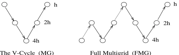
The V-Cycle (MG) Full Multigrid (FMG)

Fig. 3.Two multigrid algorithms.

The advantage of FMG over MG is that it provides a more accurate initial guess for the V-Cycle than an arbitrary or zero initial guess, at a small additional cost. (Discretization error accuracy can usually be reached in one FMG iteration, whereas several MG iterations may be required to reach the same accuracy.) However, time-dependent problems naturally provide a third option: we can exploit information available from previous time steps (the simplest approach is to use the solution at timetn as the initial guess for multigrid at timetn₊₁). We discuss this further in §7.

For an n×n×n grid, the cost of dense, banded, and sparse Gaussian elimination isO(n9_),

O(n7_{), and O(n}6_{), respectively. In contrast, one iteration of multigrid costsO(n}3_{) operations, and}

the number of iterations of multigrid required to solve the problem to discretization error accuracy is typically very small. For certain classes of problems, it can be shown rigorously that the number of iterations required is independent ofn, which implies that multigrid methods are of optimal order for these problems.

In three dimensions, the additional memory required by multigrid is not excessive. IfMh is the

memory required to describe the problem on the finest grid, then the total memory M needed by multigrid is approximately:

M =Mh+M2h+M4h+· · ·=Mh(1 +

1 8+

1

16+· · ·)≤ 8 7Mh.

Many convergence proofs can be found in the literature [1, 2, 4, 16] and are based on an analysis of the iteration matrix of the multigrid method, which for the two-grid CS scheme is given by:

G2h h =S

ν 2 h (Ih−I

h 2hL−

1 2hI

2h h Lh)S

ν 1 h ,

whereSh represents the iteration matrix for the relaxation processRh.

6. Test Problems. Our test problems are defined on the unit cube and are of the form given in equations (1) and (2). We will present results for the following two test problems.

Problem 1. For this problem, Lis chosen to be the Laplacian, i.e., in (2) we set a11=a22=a33= 1, b1=b2=c= 0.

The boundary and the initial conditions are chosen to agree with a test solution which we have chosen, namely:

u(x, y, z, t) =e−t_{sin(πx)sin(πy)sin(πz).}

Problem 2. This problem is a generalization to three dimensions of a 2D test problem that appeared in [34]. In particular,Lis a time-dependent, variable coefficient, non-self-adjoint, elliptic operator. The coefficients in (2) are defined as follows:

a11=

t

6(x+ 1)2, a22=

t

6(y+ 1)2, a33=

t 6(z+ 1)2,

b1=

−t

6(x+ 1)3, b2=

−t

6(y+ 1)3, b3=

−t

10-3 10-2 10-1 100

10-3 ₁₀-2 ₁₀-1 ₁₀0 ₁₀1 ₁₀2 ₁₀3 ₁₀4 o o

o o o

o o o

o

o

o

SIZE OF TIME STEP

MULTIGRID RESIDUAL REDUCTION RATE

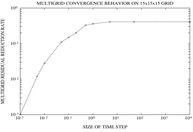
MULTIGRID CONVERGENCE BEHAVIOR ON 15x15x15 GRID

Fig. 4.Effect of varying the Crank-Nicolson time shift in Problem 2 on a15×15×15mesh.

The boundary and initial conditions are chosen to agree with the test solution which we choose as

u(x, y, z, t) =e−t2

sin((x+ 1)2+ (y+ 1)2+ (z+ 1)2).

The results which we present in§7 are for Problem 2, while the results presented in§8 are for Problem 1.

7. Sequential Behavior and Performance. In this section, we first consider the issue of step size selection for both the explicit and implicit time stepping schemes. Next, we mention several possible techniques for starting the multigrid iteration at a particular time step of an implicit scheme, and explain the approach we took. We then examine the sequential behavior and performance of the three time stepping methods we implemented, when each method uses nearly optimal step sizes. Finally, we make some comments about the effect of the time step on multigrid convergence rates.

7.1. Step Size Selection. In our experiments, we first select the spatial meshwidth ∆x, and then determine a time step ∆t that is as large as possible while maintaining a degree of accuracy at the final time point commensurate with the spatial discretization error.

An important issue regarding the time step selection arises when using the multigrid method for the implicit equations. It was noted in § 4.1 that the size of the time step chosen effects the conditioning of the elliptic equation (7). As ∆t approaches zero, the operator becomes more well-conditioned, and this is reflected in a smaller convergence factor for multigrid; this is shown in Figure 4. Naturally, we are interested in taking large time steps and it is clear that the multigrid convergence rates for the shifted elliptic operator in equation (7) is never larger than for the unshifted operatorL1_.

When solving an application problem rather than a test problem, the luxury of determining the optimal step size, either analytically or empirically, does not exist, and therefore either a fixed time step must be chosen a priori, or some type of adaptive time stepping strategy must be employed. If one has a spatial error estimate, then one could attempt to maintain maximal accuracy while taking the fewest possible time steps by exploiting the spatial error information. The structure of multigrid

methods makes it easy to estimate the accuracy of the computed solution. We outline two simple possibilities.

In the CS multigrid scheme, the solution on the 2hgrid, when transferred to the finest hgrid, can be viewed as an approximation to the error on the finest grid. In the notation of Figure 2, kchk/k¯uhkcould be used as an error estimator in the spirit of iterative improvement (e.g., [15]).

Alternatively, if the FMG and/or FAS multigrid approach is used, we have approximate solutions on each grid. The solutions on thehand 2hgrids can be combined to produce an error estimate, using either Richardson extrapolation orτ extrapolation [7].

Ideally, the spatial error estimate thus obtained would be combined with an error estimate in time, to implement adaptive time stepping. Eventually, it would be desirable to implement methods which are adaptive in both space and time for 3D parabolic problems. This question is addressed for nonlinear parabolic problems in one space dimension in [26].

7.2. Initial Guess for Multigrid. The Multigrid V-cycle solution of the discrete equations at timetn₊₁ can in principle be initialized in one of several ways, including:

• the solutionun

from the previous time step, • an initial approximation from FMG,

• use of a predictor.

Since explicit methods used as predictors typically violate their stability limits, they may excite high frequency modes in the predicted value, and therefore may create more work to be done on the fine grid of the next time step [8]; for this reason, the predictor approach may not be worthwhile.

Brandt et al. [8] argue that while the previous time step or some extrapolated approximation other than a predictor can be used, the FMG approach coupled with a variation of the V-Cycle, the

F-Cycle, is optimal. For the particular problems we have looked at, and for our implementation,

our experiments seem to indicate that the previous time step is a marginally better initialization to the V-cycle than is the FMG approach. Whether this would remain true for other problems or multigrid method formulations (e.g., if cubic interpolation is used in FMG; cf., Figure 3) remains open.

7.3. Comparisons of Explicit and Implicit Methods. We integrated the test problem, using our empirically determined nearly optimal time step, with each of the three methods to time t= 1, noting the cost of each method on a sequential computer. Note that the implicit equations were solved with the multigrid method at each time step.

Table 1 presents some results, in which we give the number of time steps required to reach a given tolerance, the cost of each step, and the total cost of all time steps, for the solution of a variable coefficient problem (Problem 2) on a 15×15×15 mesh. Table 2 presents the results of the same experiments for a 31×31×31 mesh.

The number of steps required by each of the methods to reach the final time point is dictated by the stability limit in the Forward Euler method, while accuracy considerations constrain the Backward Euler method to taking more time steps than Crank-Nicolson. However, the cost for each time step is more expensive for the implicit methods. The question then arises as to whether the explicit method is so inexpensive to apply that it can overcome the penalty imposed by the stability limit.

The results presented in Tables 1 and 2 indicate that this is not the case on sequential computers, at least when an efficient solver (multigrid in this case) is used for the implicit equations. On parallel computers this situation could change, if the explicit method ran at a much higher parallel efficiency than the implicit method. However, noting that the ratio of the total sequential times given in Table 1 for Forward Euler and Crank-Nicolson is roughly five, this would imply that the explicit method would have to achieve a parallel efficiency five times greater than the implicit method to be competitive. In this scenario, if the implicit method achieves over twenty percent parallel efficiency, then the explicit method is not likely to be competitive. As we will see in§8.1 and §8.2, we are able to achieve substantially more than twenty percent parallel efficiency, from FORTRAN, for our implementation of the Crank-Nicolson method with multigrid.

Table 1

Solution of Problem 2 on a15×15×15mesh. CPU seconds on a Convex C240 to reacht_{f inal}= 1.

Method Number of Time for Time for Accuracy Steps N 1 step N steps

Forward Euler 1010 1.87E−02 18.9 1.6E−03 Backward Euler 105 1.97E−01 20.7 2.0E−03 Crank-Nicolson 20 2.01E−01 4.0 2.6E−03

Table 2

Solution of Problem 2 on a31×31×31mesh. CPU seconds on a Convex C240 to reacht_{f inal= 1.}

Method Number of Time for Time for Accuracy Steps N 1 step N steps

Forward Euler 4040 1.51E−01 610.0 3.9E−04 Backward Euler 350 1.51E+ 00 528.5 5.0E−04 Crank-Nicolson 30 1.55E+ 00 46.5 6.2E−04

competitive with implicit methods, for sequential or coarse-grained parallel computers.

8. Performance on Advanced Computer Architectures. We have implemented a 3D multigrid solver for a class of problems that includes the elliptic problems arising at each time step of an implicit method. This solver has been interfaced with a parabolic equation integrator which implements both Backward Euler and Crank-Nicolson time stepping. The multigrid solver can use either the V-Cycle algorithm (with either zero or the previous time level solution as the initial guess) or the FMG algorithm, with weighted Jacobi smoothing, full-weighting restrictions, tri-linear interpolation, and banded Gaussian elimination for the coarse grid solves.

The FORTRAN code executes with high vector and parallel efficiency on machines such as the Alliant FX/2800, the Cray Y-MP, and also executes efficiently on the IBM RS6000, the Convex C240, and the Sun SPARC-1. The multigrid code consists of four central routines: the smoothing routine, the residual routine, and the restriction and interpolation routines. The restriction and interpolation routines consist of triply nested loops which scan through the grid functions by plane, line, and point; appropriate compiler directives must be placed in the code in order for parallelization across the planes to take place. The smoothing and residual routines, on the other hand, consist of long single loops as a result of the diagonal matrix storage scheme. These loops may need to be restructured in order for parallelization to be enabled on different architectures.

The performance figures presented below, as well as the summary in Table 3 refer to identical code, other than the insertion of necessary compiler directives mentioned above to force paralleliza-tion across planes in the restricparalleliza-tion and interpolaparalleliza-tion routines (this was automated for a number of compilers), and hand restructuring of long single loops in the smoothing and residual routines to enable parallelization in the case of the Cray Y-MP.

In what follows, we examine the parallel and vector performance on the Cray and the Alliant in detail. Table 3 summarizes these results along with the overall performance of the code on several other machines. For the results that follow in§8.1 and§8.2, we use the notions of parallel speedup SP, parallel efficiency EP, and Megaflops as performance indicators. The standard definitions for

these measures are (for a program running onP processors of a parallel computer):

SP ≡

Execution time on 1 processor

Execution time on P processors, EP ≡SP× 1

P ×100%.

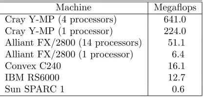
Table 3

Performance summary of the 3D parabolic multigrid solver on several architecures.

Machine Megaflops Cray Y-MP (4 processors) 641.0 Cray Y-MP (1 processor) 224.0 Alliant FX/2800 (14 processors) 51.1 Alliant FX/2800 (1 processor) 6.4

Convex C240 16.1

IBM RS6000 12.7

Sun SPARC 1 0.6

Table 4

Percentage of solution time spent in main multigrid components when solving Problem 2 on a31×31×31mesh.

Multigrid Alliant FX/2800 Cray Y-MP

Component P=1 P=14 P=1 P=4

Smoothing 76% 75% 75% 79%

Residual 14% 14% 12% 10%

Interpolation 4% 5% 8% 6%

Restriction 2% 3% 3% 3%

Coarse Grid Solve <1% <1% <1% <1%

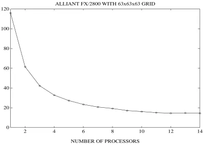
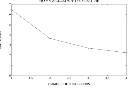
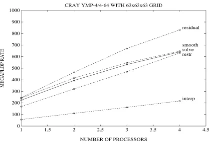
Figures 5 through 8 display the execution times, speedup, parallel efficiency for the overall solution process, and the megaflop rate breakdown for each major component in the multigrid method at one particular time step.

Figure 5 shows the reduction in execution time as more processors are used. Figure 6 shows a speedup of nearly eight on fourteen processors, which when translated to parallel efficiency in Figure 7 shows nearly sixty percent efficiency. Figure 8 shows an overall performance of over fifty megaflops on fourteen processors, and also reveals a routine that lags in performance: the interpolation routine. (Note that interpolation is only about three to eight percent of the overall solution time, and therefore does not constitute a substantial bottleneck; see Table 4.)

From these figures we can make a few observations. First, the code runs at about six megaflops on a single processor. This is somewhat disappointing, given the high peak performance of the i860 chips (thirty to forty megaflops for SAXPYs [11, 21]). Secondly, the leveling off in the parallel efficiency curve is at first glance somewhat unexpected. However, for a method like multigrid where O(N) operations are performed on data of sizeN, it is harder for the cache management algorithm to do a good job, than, say, for Gaussian elimination, where O(N3_{) operations are performed on}

O(N2_{) data. This in turn leads to greater contention for the bus, as the number of processors is}

increased.

8.2. Parallel and Vector Performance on the Cray Y-MP. Our implementation was also run on the Cray Y-MP, located at the National Center for Supercomputer Applications at the University of Illinois, Urbana-Champaign. The architecture is also a shared memory multiproces-sor, with four Cray vector processors. We used the micro-tasking facility (do-loop level) rather than macro-tasking (subroutine level) to parallelize our code. There is compiler support for some parallel programming, which is used through a compiler front-end which inserts micro-tasking (“au-totasking”) compiler directives. However, we were forced to hand nest the long single loops of the smoothing and residual routines in order for the autotasking directives to be correctly inserted by the compiler front-end; this was not necessary for the Alliant compiler.

and twenty megaflops on one processor, and over six hundred and forty megaflops on four processors. (Again, the lagging interpolation routine is revealed.)

From these figures we can see that the choice of diagonal matrix data structures paid a large dividend in performance: the smoothing and residual routines are the fastest components of the multigrid method on the Cray. Secondly, on one processor of the Cray Y-MP, we achieve over two hundred and twenty megaflops, which is nearly the peak performance of the older Cray X-MP. Finally, if an eight processor version of the Cray Y-MP had been available, a performance of over a gigaflop seems plausible, given the slope and curvature of the speedup plot on four processors in Figure 10.

9. Conclusions. We conclude by making a few observations.

First, it is clear that if the implicit equations are solved using the multigrid method, not only is the resulting method sequentially very efficient, but it can also achieve high vector and parallel efficiencies. This is of course not new [3, 13], but what can be said is that this performance is achievable from FORTRAN with very little special coding considerations.

Second, the shifted elliptic operators arising at each time step of an implicit time discretization results in rapid multigrid convergence. Furthermore, multigrid can exploit information available from previous time steps by using the previous solution as an initial guess for the multigrid V-Cycle. Third, explicit methods may achieve somewhat higher computation rates, but not enough to overcome their inherent disadvantages, at least on coarse grained parallel architectures such as the ones considered in this paper. In particular, for the methods we implemented, the implicit methods were superior even for small problems, and as the problem size grows, the superiority of the implicit methods will only increase.

Finally, although we did not implemented this idea, we feel that adaptive step-size selection will be straightforward to implement when using multigrid for the implicit equations, and lead to even greater efficiency.

Acknowledgments. Dr. Ahmed Sameh, at the Center for Supercomputing Research and Development at the University of Illinois at Urbana-Champaign, was kind enough to allow us to use the Alliant FX/2800 for some of our numerical experiments. Also, Stan Kerr at the University of Illinois’ Computing Services Organization arranged for us to have access to the Cray Y-MP at the National Center for Supercomputer Applications, also located at the University of Illinois.

REFERENCES

[1] R. E. Bank and C. C. Douglas,Sharp estimates for multigrid rates of convergence with general smoothing and acceleration, SIAM J. Numer. Anal., 22 (1985), pp. 617–633.

[2] R. E. Bank and T. F. Dupont,An optimal order process for solving finite element equations, Math. Comp., 36 (1981), pp. 35–51.

[3] E. Barszcz, T. F. Chan, D. C. Jesperson, and R. S. Tuminaro,Performance of a parallel code for the Euler equations on hypercube computers, Tech. Report NASA 102260, NASA, 1990.

[4] D. Braess and W. Hackbusch,A new convergence proof for the multigrid method including the V-cycle, SIAM J. Numer. Anal., 20 (1983), pp. 967–975.

[5] A. Brandt,Multi-level adaptive solutions to boundary-value problems, Math. Comp., 31 (1977), pp. 333–390. [6] ,Guide to multigrid development, in Multigrid Methods: Proceedings of K¨oln-Porz Conference on

Multi-grid Methods, Lecture notes in Mathematics 960, W. Hackbusch and U. Trottenberg, eds., Berlin, Germany, 1982, Springer-Verlag.

[7] ,Multigrid techniques: 1984 guide with applications to fluid dynamics, Tech. Report GMD-Studien Nr. 85, GMD, Bonn, 1984.

[8] A. Brandt and J. Greenwald, Parabolic multigrid revisited, in Third European Conference on Multigrid Methods, Bonn, Germany, 1990, Springer-Verlag.

[9] J. E. Dendy, Jr.,Two multigrid methods for three-dimensional problems with discontinuous and anisotropic coefficients, SIAM J. Sci. Statist. Comput., 8 (1987), pp. 673–685.

[10] J. J. Dongarra, J. R. Bunch, C. B. Moler, and G. W. Stewart,LINPACK Users’ Guide, SIAM, Philadel-phia, PA, 1979.

[11] T. H. Dunigan,Performance of the Intel iPSC/860 hypercube, Tech. Report ORNL/TM-11491, Oak Ridge National Laboratory, 1990.

[12] D. J. Evans,Fast ADI methods for the solution of linear parabolic partial differential equations involving two space dimensions, BIT, 17 (1977), pp. 486–491.

[14] C. I. Goldstein,Multigrid preconditioners applied to the iterative solution of singularly perturbed elliptic bound-ary value problems and scattering problems, Tech. Report BNL-37225, Brookhaven National Laboratory, 1990.

[15] G. H. Golub and C. F. Van Loan,Matrix Computations, The Johns Hopkins University Press, Baltimore, MD, second ed., 1989.

[16] W. Hackbusch,On the convergence of multi-grid iterations, Beitr¨age Numer. Math., 9 (1981), pp. 213–239. [17] ,Parabolic multi-grid methods, in Computing Methods in Applied Sciences and Engineering, VI, New

York, NY, 1984, North Holland.

[18] ,Multi-grid Methods and Applications, Springer-Verlag, Berlin, Germany, 1985. [19] W. Hackbusch and U. Trottenberg, eds., Berlin, Germany, 1982, Springer-Verlag.

[20] , eds.,Multigrid Methods II: Proceedings of the Second European Conference on Multigrid Methods held at Cologne, Berlin, Germany, 1986, Springer-Verlag.

[21] M. T. Heath, G. A. Geist, and J. B. Drake,Early experience with the Intel iPSC/860 at Oak Ridge National Laboratory, Tech. Report ORNL/TM-11655, Oak Ridge National Laboratory, 1990.

[22] M. Holst and F. Saied,Vector multigrid: An accuracy and performance study, Tech. Report UIUCDCS-R-90-1636, Numerical Computing Group, Department of Computer Science, University of Illinois at Urbana-Champaign, 1990.

[23] ,Multigrid methods for computational ocean acoustics on vector and parallel computers, in Proceedings of the Third IMACS Symposium on Computational Acoustics, New York, NY, North Holland, 1991. [24] W. H. Holter,A vectorized multigrid solver for the three-dimensional Poisson equation, Appl. Math. Comp.,

19 (1986), pp. 127–144.

[25] T. L. Jordan,A guide to parallel computation and some Cray-1 experiences, in Parallel Computations, G. Ro-drigue, ed., Academic Press, New York, NY, 1982, pp. 1–50.

[26] J. Lawson, M. Berzins, and P. M. Dew,Balancing space and time errors in the method of lines for parabolic problems, SIAM J. Sci. Statist. Comput., 12 (1991), pp. 573–594.

[27] J. G. Lewis and H. D. Simon,The impact of hardware gather/scatter on sparse gaussian elimination, SIAM J. Sci. Statist. Comput., 9 (1988), pp. 304–311.

[28] C. Lubich and A. Ostermann,Multi-grid dynamic iteration for parabolic equations, BIT, 27 (1987), pp. 217– 234.

[29] R. D. Richtmyer and K. W. Morton,Difference Methods for Initial-Value Problems, Interscience Publishers, New York, NY, second ed., 1957.

[30] K. St¨uben and U. Trottenberg,Multigrid methods: Fundamental algorithms, model problem analysis and applications, in Multigrid Methods: Proceedings of K¨oln-Porz Conference on Multigrid Methods, Lecture notes in Mathematics 960, W. Hackbusch and U. Trottenberg, eds., Berlin, Germany, 1982, Springer-Verlag. [31] C.-A. Thole and U. Trottenberg,Basic smoothing procedures for the multigrid treatment of elliptic

3d-operators, Tech. Report GMD-Studien Nr. 141, GMD, Bonn, 1985.

[32] S. Vandewalle and R. Piessens, Efficient parallel algorithms for solving initial-boundary value and time-periodic parabolic partial differential equations, Tech. Report TW 139, Department of Computer Science, K.U.Leuven, Heverlee, Belgium, 1990.

[33] ,Numerical experiments with multigrid waveform relaxation on a parallel processor, Tech. Report TW 142, Department of Computer Science, K.U.Leuven, Heverlee, Belgium, 1990.

[34] S. Vandewalle, R. Van Driessche, and R. Piessens, The parallel implementation of standard parabolic marching schemes, Tech. Report TW 125, Department of Computer Science, K.U.Leuven, Heverlee, Bel-gium, 1989.

0 20 40 60 80 100 120

2 4 6 8 10 12 14

o

o

o

o

o o

o _o

o _o

o o o o

NUMBER OF PROCESSORS

SOLVE TIME

ALLIANT FX/2800 WITH 63x63x63 GRID

Fig. 5.Execution times over 14 processors on the Alliant FX/2800.

2 4 6 8 10 12 14

2 4 6 8 10 12 14

o o

o o

o o

o o

o o

o o o o

NUMBER OF PROCESSORS

SPEEDUP

ALLIANT FX/2800 WITH 63x63x63 GRID

0 10 20 30 40 50 60 70 80 90 100

2 4 6 8 10 12 14

o o o o o o o o o o o o o o

NUMBER OF PROCESSORS

PARALLEL EFFICIENCY

ALLIANT FX/2800 WITH 63x63x63 GRID

Fig. 7.Parallel efficiency over 14 processors on the Alliant FX/2800.

0 10 20 30 40 50 60

2 4 6 8 10 12 14 16 18

o o o o o o o o o o o o o o o o o o o o o o o o o o o o o o o o o o o o o o o o o o o o o o o o o o o o o

o o o

o o o o o o o o o o

o o o o

solve residual smooth

restr

interp

NUMBER OF PROCESSORS

MEGAFLOP RATE

ALLIANT FX/2800 WITH 63x63x63 GRID

0 1 2 3 4 5 6 7

1 1.5 2 2.5 3 3.5 4

o

o

o

o

NUMBER OF PROCESSORS

SOLVE TIME

CRAY YMP-4/4-64 WITH 63x63x63 GRID

Fig. 9.Execution times over 4 processors on the Cray Y-MP.

1 1.5 2 2.5 3 3.5 4

1 1.5 2 2.5 3 3.5 4

o

o

o

o

NUMBER OF PROCESSORS

SPEEDUP

CRAY YMP-4/4-64 WITH 63x63x63 GRID

0 10 20 30 40 50 60 70 80 90 100

1 1.5 2 2.5 3 3.5 4

o

o

o

o

NUMBER OF PROCESSORS

PARALLEL EFFICIENCY

CRAY YMP-4/4-64 WITH 63x63x63 GRID

Fig. 11.Parallel efficiency over 4 processors on the Cray Y-MP.

0 100 200 300 400 500 600 700 800 900 1000

1 1.5 2 2.5 3 3.5 4 4.5

o

o

o

o

o

o

o

o

o

o

o

o

o

o

o

o

o

o

o

o

solve residual

smooth

restr

interp

NUMBER OF PROCESSORS

MEGAFLOP RATE

CRAY YMP-4/4-64 WITH 63x63x63 GRID