Vlasov simulations of trapping and loss of auroral electrons

www.ann-geophys.net/33/279/2015/ doi:10.5194/angeo-33-279-2015

© Author(s) 2015. CC Attribution 3.0 License.

Vlasov simulations of trapping and loss of auroral electrons

H. Gunell1, L. Andersson2, J. De Keyser1, and I. Mann3,4

1_{Belgian Institute for Space Aeronomy, Avenue Circulaire 3, 1180 Brussels, Belgium}

2_{University of Colorado, Laboratory for Atmospheric and Space Physics, Boulder, CO 80309, USA} 3_{EISCAT Scientific Association, P. O. Box 812, 981 28 Kiruna, Sweden}

4_{Department of Physics, Umeå University, 901 87 Umeå, Sweden} Correspondence to: H. Gunell (herbert.gunell@physics.org)

Received: 27 October 2014 – Revised: 4 February 2015 – Accepted: 12 February 2015 – Published: 4 March 2015

Abstract. The plasma on an auroral field line is simulated using a Vlasov model. In the initial state, the acceleration re-gion extends from one to three Earth radii in altitude with about half of the acceleration voltage concentrated in a sta-tionary double layer at the bottom of this region. A popu-lation of electrons is trapped between the double layer and their magnetic mirror points at lower altitudes. A simulation study is carried out to examine the effects of fluctuations in the total accelerating voltage, which may be due to changes in the generator or the load of the auroral current circuit. The electron distribution function on the high potential side of the double layer changes significantly depending on whether the perturbation is toward higher or lower voltages, and there-fore measurements of electron distribution functions provide information about the recent history of the voltage. Electron phase space holes are seen as a result of the induced fluctu-ations. Most of the voltage perturbation is assumed by the double layer. Hysteresis effects in the position of the double layer are observed when the voltage first is lowered and then brought back to its initial value.

Keywords. Magnetospheric physics (Auroral phenomena; Electric fields) – Space plasma physics (Numerical simula-tion studies)

1 Introduction

Auroral optical emissions are caused by electrons that have been accelerated by electric fields that are parallel to the mag-netic field. These parallel fields have been measured, for ex-ample, by the S3-3 (Mozer et al., 1977), Viking (Lindqvist and Marklund, 1990), Polar (Mozer and Kletzing, 1998), and FAST (Ergun et al., 2002) satellites. The parallel

elec-tric fields can be concentrated in thin elecelec-tric double layers as was proposed by Alfvén (1958). Their presence has been confirmed by satellite-based measurements using the S3-3 (Temerin et al., 1982), Polar (Mozer and Kletzing, 1998), and FAST (Ergun et al., 2002) spacecraft. The latter also found strong double layers in the downward current region (Ander-sson et al., 2002). FAST data has also been used to study electron phase space holes and electromagnetic radiation in the vicinity of double layers (Pottelette et al., 2014). Exten-sive studies of parallel electric fields and their role in auroral acceleration have been performed using the Cluster space-craft (Marklund et al., 2001, 2011; Sadeghi et al., 2011; Li et al., 2013). Forsyth et al. (2012) used Cluster data to study a case with a time varying acceleration voltage and found that the majority of the change,1V, was assumed below the spacecraft altitude of about 4700 km.

Song et al. (1992) derived a stability criterion for double layers in a converging magnetic field, showing that a stable double layer position is possible when electrons are accel-erated into a stronger magnetic field. Ergun et al. (2000b) used a static model to find solutions to the Vlasov–Poisson system over a distance of a few Earth radii along an auroral flux tube. The Vlasov equation was used in plasma physics by Vlasov (1938), although an equation of the same form had been used earlier to study the motion of stars (Jeans, 1915). Poisson’s equation was published by Poisson (1813). Hwang et al. (2009) studied ion heating and outflow using a Vlasov simulation model of the downward current region. Other ways of modelling include drift-kinetic simulations that have shown electron heating and parallel electric field related to shear Alfvén waves (Watt et al., 2004). Vlasov sim-ulations of double layer formation in unmagnetised plasmas were performed by Singh (1980), who also found electron phase space holes on the high potential side of the double layer (Singh, 2000).

It was pointed out by Persson (1966) that a unique po-tential profileV (z)cannot always be found. Whipple (1977) introduced an effective potential U (z)=qV (z)+µB(z), whereq is the particle charge,µits magnetic moment and

B the magnetic flux density. If there is a maximum inU (z)

between the source of the particle population and the point in space under consideration, call itz=z1, the distribution function cannot be determined uniquely by the local V (z1) and B(z1). With a maximum inU (z), knowledge ofV (z) andB(z)for all points betweenz1and the source is required. Chiu and Schulz (1978) showed that the condition for there being no maximum is that dV /dB >0 and d2V /dB2≤0, and they went on to consider only steady state solutions that fulfil that condition. If, instead of a maximum, a minimum exists inU (z), this constitutes an effective potential well, in which particles can be trapped. The trapped particle popula-tions inhabit a region of phase space from which they can-not reach the system boundaries for the given shape ofU (z). Equivalently, this region of phase space cannot be reached by particles entering through the system boundaries. Thus, if a steady state solution is sought, assumptions must be made about the trapped particle populations. Such assump-tions were made in previous studies by, for example, Chiu and Schulz (1978) and Ergun et al. (2000b). The influence of the trapped electrons on V (z)was studied by the latter and by Boström (2004) by varying the density assumed for the trapped population.

Since auroral potential differences are changing with time, we allow the potential to evolve, and particles can be caught and trapped during the formation of a potential profile. Gunell et al. (2013a) found that an electron population be-came trapped between a double layer and the magnetic mir-ror field at lower altitudes. It has also been found that fluc-tuations are an important influence on the electron distri-butions, leading to electron conics such as those observed by the Viking satellite (André and Eliasson, 1992; Eliasson

et al., 1996). Temporal variations of the potential have been observed by the Cluster spacecraft (Marklund et al., 2001, 2011; Sadeghi et al., 2011; Forsyth et al., 2012). In this paper, we perform numerical experiments on a system that contains trapped electrons in order to study how they are trapped and how they can be released again.

2 Simulation model

We study the trapped and precipitating electron populations through the use of a Vlasov simulation code that is one-dimensional in space and two-one-dimensional in velocity space (Gunell et al., 2013a). This model was used to model the plasma on an auroral magnetic field line and also to inves-tigate how auroral acceleration can be simulated in a labora-tory experiment (Gunell et al., 2013b).

In this model, the distribution function is f (z, vz, µ, t ), where z is the spatial coordinate parallel to the magnetic field,vz is the parallel velocity, andµ=mv⊥2/2B(z)is the

magnetic moment. The magnetic moment is a constant of motion, and therefore we haveµ˙ =0. The Vlasov equation (Vlasov, 1938) that needs to be solved for our system is (Gunell et al., 2013a)

∂f ∂t +vz

∂f ∂z+

1

m

qE−µdB

dz +mag

_∂f

∂vz

=0. (1)

In the gravitational accelerationagonly the component paral-lel to the magnetic field is included. The electric field is found by solving a Poisson type equation (Poisson, 1813) that has been adapted to the geometry of the problem at hand. The equation used here is (Gunell et al., 2013a)

d

dz

_B

S B E

= ρl

S, (2)

whereSis the cross section of the flux tube at the point where

B=BS. The line chargeρlon the right hand side of Eq. (2) is the charge per unit length of the flux tube. It is computed by integrating the distribution function over velocity space and forming the sum over all speciess(Gunell et al., 2013a)

ρl=

X

s

qs

Z

fs(vz, µ)dµdvz. (3)

In Eq. (2), the constant=0rincludes an artificial relative dielectric constantr. This has been introduced for compu-tational reasons; because λD∼

√

r and ωp∼1/ √

r it al-lows the simulation to be run with a longer time step on a coarser spatial grid. Thus the system can be filled with plasma quickly at a highrvalue, and a time accurate sim-ulation can subsequently be run with a lower r. The nu-merical experiments presented in this article were run at

For relativistic particles, instead of conservation ofµ, the conserved quantity is (Alfvén and Fälthammar, 1963)

µ0= p 2 ⊥

2m0B =γ

2_m 0v⊥2

2B , (4)

wherem0is the particle mass at rest, and γ is the Lorentz factor. In the simulations described in the following sections, the electrons that have their source at the magnetospheric end of the system are treated relativistically, and we there-fore write the distribution as a function ofµ0rather than µ

for this species. For further details about the model we refer the reader to our previous paper (Gunell et al., 2013a).

3 Initial state

Using a dipole model of the magnetic field, we have sim-ulated the plasma on a flux tube of the L=7 shell from the equatorial magnetosphere, where z=0, down to the ionosphere, where z=5.5×107m. At the magnetospheric boundary of the system we impose a Maxwellian plasma with kBTe/e=500 V and kBTi/e=2500 V. At the iono-spheric boundary we assume Maxwellian distributions with

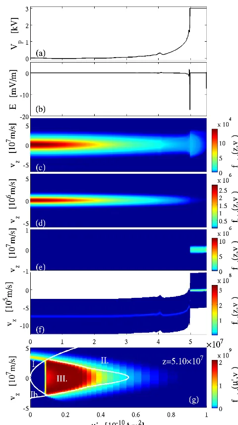
kBT /e=1 V for both electrons and ions. All the ions in-cluded here are protons. We treat particles that have their sources at the two ends of the system as different species, and thus we have four species in the simulation: electrons from the magnetosphere; protons from the magnetosphere; electrons from the ionosphere; and protons from the iono-sphere. The initial state of the numerical experiments that are reported in Sect. 4 is a simulation run with a voltage of 3 kV over the system. The initial state is illustrated in Fig. 1; Fig. 1a shows the plasma potential, and it is seen that about half of the voltage falls in a double layer at z=5×107m. The position can be determined as the position of the large negative spike in Fig. 1b.

While half of the total voltage is concentrated in a dou-ble layer, the other half is in an outstretched region above it. Similar weak parallel electric fields have been found in simulations of Alfvén waves (Vedin and Rönnmark, 2008; Watt and Rankin, 2009). Our simulation is completely elec-trostatic and can therefore not simulate Alfvén waves. How-ever, the electron time scale is faster than the time scale of Alfvén waves. Thus, an electrostatic equilibrium may be es-tablished in a few seconds, and that equilibrium be perturbed by Alfvén waves on time scales of tens of seconds or min-utes.

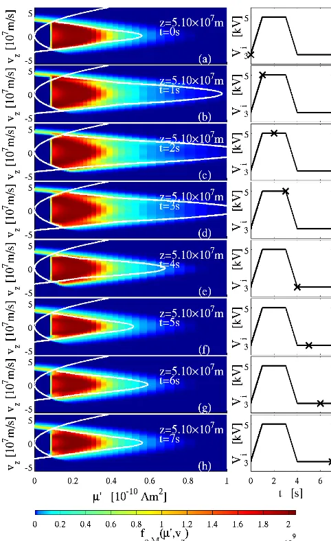
The simulation leading to the initial state in this paper dif-fers from the final state of the simulation by Gunell et al. (2013a) in that theµ0resolution of the magnetospheric elec-trons has been improved, as can be seen in Fig. 1g, which shows the distribution function f (µ0, vz) near the double layer on its high potential side atz=5.1×107m. Here, and in all the following figures that show f (µ0, vz), the white lines indicate the boundaries of different phase space

re-Figure 1. Initial state of the system for all three numerical

ex-periments. (a) Plasma potential. (b) Electric field. (c)–(f) Phase space densityf (z, vz)for (c) magnetospheric electrons; (d) magne-tospheric ions; (e) ionospheric electrons; and (f) ionospheric ions.

(g) Phase space densityfe,M(µ0, vz)for the electrons from the mag-netosphere atz=5.10×107m, which is close to the double layer on its high potential side. The phase space regions separated by the white lines are I: precipitating electrons; Ib: up-going electrons that will reflect and then precipitate; II: electrons which can reach the equator; and III: trapped electrons. The unit forfe,M(µ0, vz) is m−6A−1s. In panels (c)–(f), the colour scales have been nor-malised so that integrals over allvzgivens/B. The unit forf (z, vz) is m−4T−1s.

after first being reflected by the electric field. In region II, the electrons can reach the equator, and region III contains elec-trons that are trapped between the magnetic mirror and the potential drop. The lines are calculated according to Gunell et al. (2013a), and take into accountV andB at allzpoints between the point shown, z=5.1×107m in this case, and the boundary in question. Given enough time, electrons can reach the ionosphere if

µ0≤ min z1<z≤Lz

1

B(z)−B1

q (V1−V (z))+ mv_z2₁

2

!

, (5)

and they can reach the magnetospheric end of the system if

µ0≥ max 0≤z<z1

1

B(z)−B1

q (V1−V (z))+ mv_z2₁

2

!

, (6)

where z=z1 is the point in space under consideration, V (z1)=V1,B(z1)=B1, and z=Lz is thezcoordinate of the ionosphere (Gunell et al., 2013a). A reduced distribution functionf (z, vz), where we have integrated over theµ0 di-mension, is shown in Fig. 1c–f for each species.

The relevant time scales can be estimated by computing approximate transit times for a few typical particles. For a magnetospheric electron with an energy of 500 eV it takes 3.8 s to cover the distance of 5×107m to the double layer, and having been accelerated to 3 keV in the double layer, a precipitating electron traverses the high potential side to the ionosphere in 0.15 s. It takes a 2.5 keV ion 72 s to move from the magnetospheric end of the system to the double layer. Ions of ionospheric origin that are accelerated to 3 keV in the double layer reachz=0 in 66 s.

4 Numerical experiments

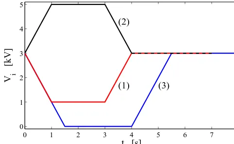
Starting from the initial state described in Sect. 3, we have performed three numerical experiments where the total volt-age imposed on the system was changed during the simu-lation run. The voltage as a function of time for the three experiments is illustrated in Fig. 2.

In experiment 1 the voltage was first decreased from 3 kV to 1 kV during one second, kept constant at 1 kV for two sec-onds, increased back to 3 kV during one second, and then the simulation was run at 3 kV for another three seconds until

t=7 s. Experiment 2 is the opposite of experiment 1, that is to say, the voltage was first increased to 5 kV and sub-sequently brought back down to 3 kV. In experiment 3 the voltage was brought down all the way to 0 V before it was increased again to 3 kV.

4.1 Experiment 1

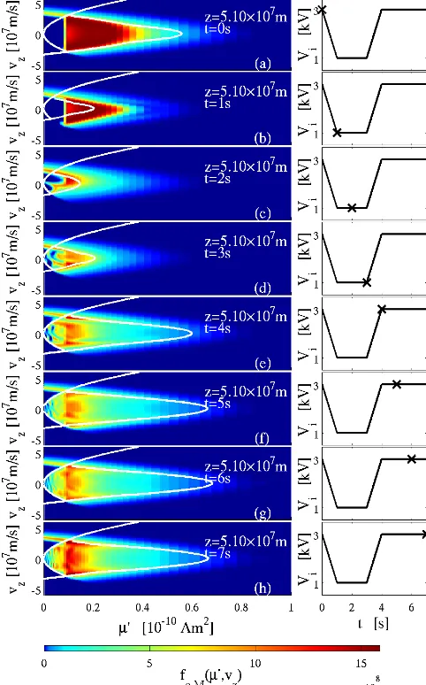
Figure 3 shows the phase space densityfe,M(µ0, vz)in ex-periment number 1 at z=5.1×107m, which is a position close to the double layer on its high potential – low altitude

0 1 2 3 4 5 6 7 8

0 1 2 3 4 5

t [s]

V i

[kV]

(1) (2)

(3)

Figure 2. The total voltage imposed on the simulated flux tube as a

function of time for the three different numerical experiments.

– side. Panels (a)–(h) show one distribution function per sec-ond, starting with the distribution in the initial state. To the right of each panel is a time profile of the total voltage over the field line with the voltage at the time for which the distri-bution is shown marked “×”.

Att=0 there was one population of precipitating elec-trons and one of trapped elecelec-trons. These trapped elecelec-trons were only present forµ0_&8×10−12A m2. The voltage was ramped down linearly from 3 kV to 1 kV, which was the volt-age att=1 s. It is seen in Fig. 3b that the phase space region populated by electrons had shrunk somewhat att=1 s com-pared to the state att=0, and that the precipitating electrons had become slightly slower invz. However, the more obvi-ous change is that the boundaries between the different phase space regions, shown by the white lines, moved. At the lower voltage the region of phase space where electrons could reach the ionosphere was smaller, the region where electrons could reach the magnetosphere larger, and the part of phase space that contained the trapped electrons had undergone the great-est diminution of them all.

The electrons that att=1 s had found themselves in the region where they were allowed to reach the magnetosphere were lost during the next two seconds while the voltage was kept at 1 kV, and it can be seen that the phase space density in this region decreased fort=2 s andt=3 s, in panels (c) and (d) respectively, compared to the initial state. It is also seen that electrons had entered the previously empty region that can contain trapped electrons at lowµ0.

Figure 3. Phase space densityfe,M(µ0, vz), in units of m−6A−1s, in experiment number 1 atz=5.1×107m for different times (on per second) are shown in the left-hand column. The time is indicated on each panel, and to the right that time is marked on a diagram of the total voltage applied over the system.

highest phase space density of the initial state in the ap-proximately triangular region betweenµ0≈8×10−12A m2 andµ0≈4×10−11A m2was, however, not recovered com-pletely. There was some increase in the phase space density forµ0.2×10−11A m2when the voltage was constant in the interval 4 s≤t≤7 s due to electrons moving in thez dimen-sion. Asµ0is a constant of motion, there can be no flux in theµ0dimension; a flux in thevzdimension, corresponding to electron acceleration, would be possible in principle, but no signs of such an acceleration can be seen in Fig. 3e–h. The electrons that appeared at lowµ0values when the volt-age was lowered remained there throughout the run of the simulation.

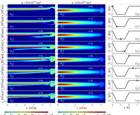
To illustrate the electron motion along the magnetic field, Fig. 4 shows distribution functionsfe,M(z, vz)for electrons

of magnetospheric origin. The left-hand column (Fig. 4a) shows a distribution that has been integrated overµ0<8× 10−12A m2, and the mid column (Fig. 4b) shows the inte-grated distribution forµ0≥8×10−12A m2. The colour scales have been normalised so that integrals over allvzyield partial density divided by magnetic field, that is to say,

Z

fe,M(z, vz)dvz=np(z)/B(z),

wherenp(z) denotes the partial density of magnetospheric electrons for theµ0 range in question. The vast majority of the electrons represented by the initial distribution shown in Fig. 4a0 were precipitating. Only a small fraction was re-flected by the magnetic mirror field and accelerated toward the double layer, where the electrons were slowed down. Then they were further decelerated by the weaker electric field at higher altitude until they returned downward to the double layer again. Thus, they were trapped between the magnetic mirror and the potential structure, specifically the part of the potential structure which was situated in an ex-tended weak field region above the double layer. For the higherµ0 range shown in Fig. 4b0there were also electrons at lower|vz|that were trapped between the magnetic mirror and the double layer electric field. This can be seen by the sharp edge at the double layer position.

As the voltage was lowered, the potential drop located in the double layer decreased, but it did not disappear com-pletely. This can be seen in Fig. 5a, where the green curve shows the initial potential profile and the red curve the po-tential att=1 s in experiment 1. As a result we see that part of the trapped population had been lost att=2 s, shown in Fig. 4b1, and as it takes some time for the electrons to turn around and leave the high potential side of the double layer, this population continued during the interval 1 s≤t≤3 s, when the voltage was constant at 1 kV in Fig. 4b2−3. In the lowµ0 range, electrons were reflected by the magnetic mir-ror, and as the voltage had been decreased they were not de-celerated as much in the double layer as in the initial state. Therefore there is a gap between the upgoing and downgo-ing populations in Fig. 4a2forz.5×107m. There was also a part of the lowµ0electron population that did not pass back through the double layer toward lowerzvalues and instead got trapped on the high potential side. These were the same particles as those that are seen filling the trapped particle re-gion forµ0.8.0×10−12A m2in Fig. 3c–h.

Figure 4. Partial phase space densityfe,M(z, vz)of magnetospheric electrons for experiment number 1. (a) Phase space density integrated over 0≤µ0<8.0×10−12A m2. (b) Phase space density integrated over 8.0×10−12A m2≤µ0<max(µ0)=7.0×10−9A m2. The colour scales have been normalised so that integrals over allvzare equal tonp/B, wherenpdenotes the partial density of magnetospheric electrons for theµrange in question, and the unit forfe,M(z, vz)is m−4T−1s. (c) Voltage as a function of time with the voltage for each row indicated by “×”. The subscript of the panel label indicates the number of seconds for which the distribution function is shown in that panel.

Fig. 3b and c – and here the accelerated electrons that were in the precipitating region for the distributions shown in Fig. 3 had been decelerated into the trap. The reason for this is the fluctuations that appeared as a result of the imposed mod-ulation of the voltage. Figure 6c shows the total voltage as a function of time (blue curve) together with the plasma potentials at two points near the double layer that initially both were on its low potential side, namelyz=4.92×107m (black curve),z=4.975×107m (red curve). When the volt-age first was lowered, all three curves decreased, but there was a rebound forz=4.92×107m so that att=1 s, the po-tential there was higher than atz=4.975×107m. This can also be seen by the dip in the red curve in Fig. 5a between the two vertical dashed lines in that figure. The oscillation that

ensued peaked at a potential near 2 kV forz=4.92×107m shortly beforet=1.5 s. After that, the oscillation decayed, and the contribution from the increase of the voltage between

t=3 and 4 s to this oscillation was smaller than that of the initial voltage decrease. The red curve showing the potential atz=4.975×107m attaches itself to the blue curve around

t=2 s, showing that the double layer moved toward lowerz

values so thatz=4.975×107m was on the high potential side aftert=2 s. The peak of the black curve corresponds to an electric field that was directed in the positivezdirection, and that is what decelerated the electrons in Fig. 6a.

3 3.5 4 4.5 5 5.5 0

0.5 1 1.5 2 2.5 3 3.5 4 4.5 5

z [107m]

V p

[kV]

(a)

Initial

exp. 1

exp. 2

exp. 3

−3 −2 0 2

−3 −2 −1 0 1 2

ΔV tot [kV]

Δ

V [kV]

(b)

−3 −2 0 2

0 0.1 0.2 0.3 0.4 0.5 0.6 0.7 0.8 0.9 1

ΔV

tot [kV] (c)

low alt.

high alt.

DL

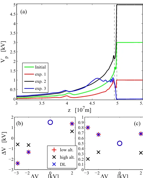
Figure 5. Distribution of1V. (a) Plasma potential as a function of

zfor the initial state (green) and the mean of the plasma potential during 0.1 s aftert=1 s for experiments 1 (red) and 2 (blue) andt= 1.5 s for experiment 3 (blue), i.e. when the respective target voltages were first reached. The left vertical dashed line is located atz= 4.94×107m where the initial plasma potential was 1500 V. The right vertical dashed line is located atz=4.99×107m. (b) The part of1Vbelow (red “+”) and above (black “×”)z=4.94×107m and the part across the double layer (blue “×”), all plotted versus the total1V. The blue circle shows the initial potential atz=4.94× 107m. (c) The same quantities as in (b), but with the vertical axis normalised to the total1V.

being reflected by the magnetic mirror field are seen, and in the centre of the image electrons were reflected by the re-versed electric field that existed in this region during the lo-cal potential peak shown by the black curve in Fig. 6c. This created two beam-like populations moving in the negativez

direction. These beams can be seen at t=2 s as the some-what complicated structure at negativevzvalues in Fig. 4a2.

4.2 Experiment 2

In experiment 2 the voltage was first increased from 3 kV to 5 kV, held constant there for 2 s and then decreased back to 3 kV, where it was maintained until t=7 s. Figure 7 shows the phase space densityfe,M(µ0, vz)in experiment 2 at z=5.1×107m, which is a position close to the double

Figure 6. Illustration of the effect of a time dependent

poten-tial profile on the particle distributions. (a) Phase space density

fe,M(µ0, vz), in units of m−6A−1s, in experiment 1 atz=5.1× 107m andt=1.5 s. (b) Partial phase space densityfe,M(z, vz), in units of m−4T−1s, of magnetospheric electrons for experiment 1, integrated over 0≤µ0<8.0×10−12A m2. (c) Plasma potential as a function of time forz=4.92×107m (black),z=4.975×107m (red), and at the ionosphere, i.e.z=5.5×107m, (blue).

layer on its high potential side. This is the same position that was shown for experiment 1 in Fig. 3.

As the voltage was increased, the boundary of the trapped electron region expanded both toward largerµ0 and larger |vz|values. The phase space density is seen to have increased just inside the parabola in Fig. 7b, both at its tip on the right-hand side of the image and for 1×10−11A m2_.µ0_.3× 10−11A m2. The electrons that were trapped by the expan-sion of the trapped particle region had entered the high po-tential side of the double layer, and after being reflected by the magnetic mirror they encountered a higher electrostatic potential barrier due to the increased voltage – as is shown by the plasma potential at t=1 s in Fig. 5a (black curve) – which prevented their return to the low potential side. When the voltage subsequently was returned to 3 kV again the newly trapped electrons were released from the trap.

In Fig. 7f–h a two-peaked distribution has developed in the range 8.0×10−12A m2_.µ0.1.4×10−11A m2with its peaks at |vz| ≈1.3×107m s−1. Thus the distribution dis-plays different behaviour for low, intermediate and high

µ0 values. In order to visualise the electron motion in the

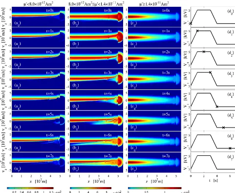
z and vz dimensions, partial fe,M(z, vz) distributions are shown in Fig. 8 for three different µ0 ranges, namely 0≤ µ0<8.0×10−12A m2in Fig. 8a, 8.0×10−12A m2≤µ0<

1.4×10−11A m2 in Fig. 8b, and 1.4×10−11A m2≤µ0<

Figure 7. Phase space densityfe,M(µ0, vz), in units of m−6A−1s, in experiment number 2 atz=5.1×107m for different times (on per second) are shown in the left-hand column. The time is indicated on each panel, and to the right that time is marked on a diagram of the total voltage applied over the system.

The initial distribution for µ0<8.0×10−12A m2 in Fig. 8a0is the same as that in Fig. 4a0, as both experiments started from the same initial state. Most of the electrons were precipitating, and the small fraction that was not can be seen to be trapped between the magnetic mirror and the potential structure above the double layer. After the voltage was in-creased, the part of this small trapped distribution that was located above the double layer was lost, as an increased ac-celeration in the double layer allowed them to precipitate. The black curve in Fig. 5a shows the plasma potential at

t=1 s in experiment 2, and it is seen that the double layer voltage increased when the total voltage was raised. After the voltage was returned to 3 kV the region that originally contained the trapped electrons was filled anew. The distri-bution betweenz=4×107m andz=5×107m was more

structured att=7 s than the original distribution, and that is a result of the potential structure that appeared in that region after the return of the total voltage to 3 kV. Similar structur-ing is also seen for the intermediate and highµ0 ranges. A fraction of the lowµ0electron distribution can also be seen returning toward the magnetospheric side of the system in Fig. 8a6and a7. This was caused by the decreasing double layer voltage during the lowering of the total voltage between

t=3 s andt=4 s. Electrons were accelerated towards higher

zby a high double layer voltage, then they were reflected by the magnetic mirror, and when they reached the double layer again its voltage had decreased, enabling them to reach the magnetosphere.

This last phenomenon can also be seen in Fig. 8b5−7 for the intermediate µ0 range. The initial distribution in this range was symmetrical with respect tovz=0 (Fig. 8b0). At the higher voltage in Fig. 8b1−3 the negative vz part was diminished as the higher voltage allowed more electrons to precipitate rather than be reflected. The initial symmetry did not return completely during the simulation run. When the voltage had been returned to 3 kV att=4 s the changed po-tential profile caused structuring and there were fluctuations causing heating of the electrons moving in the negativez di-rection. The double-peaked distribution for intermediateµ0

that was noticed in Fig. 7f–h also appears in Fig. 8b5−7. Examining a cross section of the distribution in Fig. 8b7at z=5.1×107m we find peaks atvz= ±1.3×107m s−1, that is to say, in the same place as in Fig. 7h. The peak describes a semicircle in thez–vzplane forz >5×107m in Fig. 8b7. In fact, a semicircle of varying thickness is present in all the Fig. 8b panels. The final thickness and radius with the peaks atvz= ±1.3×107m s−1forz=5.1×107m are a result of the outer – high energy – part of the semicircle, being re-leased through the double layer toward lowerzvalues after the voltage decrease. The thus released population is visible in Fig. 8b4aroundz=4.9×107m andvz= −1×107m s−1. It arrives on the low potential side at lower|vz|due to decel-eration in the double layer.

4.3 Experiment 3

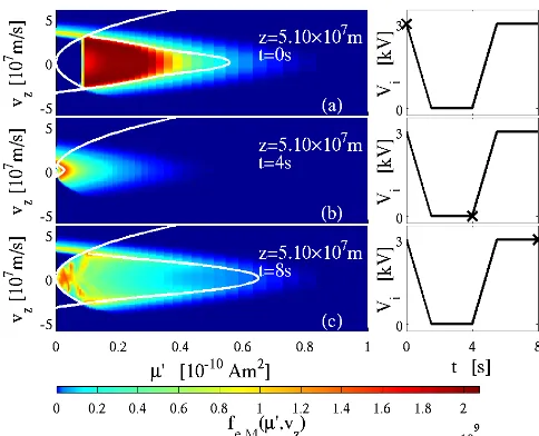
Experiment 3 started from the same initial state as the other two experiments. It followed experiment 1, but differed from it in that the voltage was brought down all the way to zero before returning to its initial value of 3 kV. Figure 9 shows the phase space densityfe,M(µ0, vz)in experiment 3 atz= 5.1×107m, which is a position close to the double layer on its high potential side. This is the same position that is shown for experiments 1 and 2 in Figs. 3 and 7, respectively. The results of experiment 3 are similar to those of experiment 1. Figure 9 shows the initial state and the distributions att=4 and 8 s, which is enough to show the differences between the two experiments.

Figure 8. Partial phase space densityfe,M(z, vz)of magnetospheric electrons for experiment number 2. (a) Phase space density integrated over 0≤µ0<8.0×10−12A m2. (b) Phase space density integrated over 8.0×10−12A m2≤µ0<1.4×10−11A m2. (c) Phase space density integrated over 1.4×10−11A m2≤µ0<max(µ0)=7.0×10−9A m2. The colour scales have been normalised so that integrals over allvz are equal tonp/B, wherenpis the partial density in theµ0range in question, and the unit forfe,M(z, vz)is m−4T−1s. (d) Voltage as a function of time with the voltage for each row indicated by “×”. The subscript of the panel label indicates the number of seconds for which the distribution function is shown in that panel.

region did not disappear completely is due to fluctuations that created a minimum in the plasma potential of Vp= −58 V at z=4.93×107m at t=4 s. The speed of the precipi-tating particles was also lower here than in experiment 1. At the end of the simulation run, when t=8 s, electrons had become trapped in the previously empty region at low

µ0_.8×10−12A m2. The phase space density was somewhat higher in this region of Fig. 9c than in the corresponding re-gion of Fig. 3h for experiment 1. The phase space density in the part of the trapped region aboveµ0=8×10−12A m2 was lower at the end of experiment 3 than at the end of ex-periment 1, due to the former being more thoroughly

emp-tied when the voltage was reduced to zero rather than only to 1 kV.

Figure 10 shows partial distribution functionsfe,M(z, vz) for electrons of magnetospheric origin in experiment 3. The division atµ0=8.0×10−12A m2is the same as that in Fig. 4, and like in Fig. 9 we have only includedt=0,4, and 8 s. This figure serves to emphasise the differences between ex-periments 1 and 3, and it confirms that the trapping of lowµ0

electrons and the emptying of the highµ0region on the high potential side of the double layer were both more efficacious in experiment 3 than in experiment 1.

Figure 9. Phase space densityfe,M(µ0, vz), in units of m−6A−1s, in experiment number 3 atz=5.1×107m fort=0,4,and 8 s are shown in the left-hand column. The time is indicated on each panel, and to the right that time is marked on a diagram of the total voltage applied over the system.

toward lower z values. This happened due to the shape of the potential profile at t=4 s, which is shown by the blue curve in Fig. 5a. When the voltage was lowered all the way to zero, the double layer shifted polarity so that it att=4 s was accelerating electrons away from Earth.

4.4 Comparison between the experiments

The change in voltage first imposed on the system was1V = −2 kV in experiment 1,1V = −3 kV in experiment 3, and

1V = +2 kV in experiment 2. Figure 5a shows the plasma potential as a function ofzfor the initial state and the mean of the plasma potential during 0.1 s after the target volt-ages of the respective experiments were reached. In order to make a quantitative assessment of how the plasma as-sumes the changed voltage we define a reference point at

z=4.94×107m, which is where the initial plasma poten-tial was 1500 V, and it is shown by the left vertical dashed line in Fig. 5a. The right vertical dashed line is located at

z=4.99×107m, and we shall take the double layer voltage to be the potential drop between those two vertical dashed lines. The positions of these lines were chosen to accommo-date the double layer in all three cases, and the distance be-tween them is therefore larger than the width of the double layer, which was approximately 180 km in the simulation of the initial state. In Fig. 5b the part of1V that is assumed at low altitude – defined asz >4.94×107m – is shown together with the high altitude part, that is to say,z <4.94×107m. The part of1V assumed by the double layer is also shown in the figure, and for reference the circle shows the initial plasma potential at the reference point, which was 1500 V.

In Fig. 5c the values shown in Fig. 5b have been normalised to the total1V for the respective experiment, and the initial plasma potential at the reference point, shown by the circle, has been normalised to the initial total voltage.

In experiment 1, 67 % of1V was assumed below the ref-erence point; in experiment 2 that value was 68 %; and in experiment 3, 80 % of 1V fell below the reference point. Furthermore, it is seen that the part of1V which was be-low the reference point was almost completely assumed by the double layer, and the plasma potential changed only a few volts over the distance from the double layer to the iono-sphere. Therefore, that part of the plasma potential curves in Fig. 5a is flat on the scale shown.

Figure 11 shows the plasma potential at the end of the simulations as functions ofz for the three experiments to-gether with the initial plasma potential. Panel (a) shows the fullzrange and panel (b) shows the region around the double layer. In experiment 2, where the voltage excursion was to-ward higher values, the double layer was at the same position in the final as in the initial state. In the two other experiments, where the voltage was decreased, the double layer moved toward higher altitudes at the end of the simulation runs. This hysteresis effect was largest in experiment 3, which had the largest|1V|of all three experiments. The double layer moved 370 km in experiment 3.

In all three experiments fluctuations in the plasma poten-tial are seen in Fig. 11 at altitudes just above the double layer. This region extends to higher altitudes in experiment 2 than in the other two. In the region where these waves appeared, holes in the electron phase space can also be seen in Fig. 8 fort≥5 s.

Figure 12 shows the phase space density of magneto-spheric electrons and ionomagneto-spheric ions in experiment 2 in panels (a) and (b) respectively for time t=5 s. Panel (c) shows the plasma potential att=4.9 s (red line) andt=5 s (black line), and panel (d) shows the electric field at these same times. In panels (a) and (b) the distribution function has been integrated over the completeµrange, and all pan-els show thezrange 4.5×107≤z≤4.9×107. The ion beam in the region shown was formed through acceleration in the double layer when the total voltage was increased to 5 kV and it was therefore faster here than at lowerzvalues.

Each electron hole in Fig. 12a corresponds to a perturba-tion of the ion beam in Fig. 12b and a positive potential peak in Fig. 12c, showing that the hole was positively charged. The velocity with which the hole atz=4.8×107m moved was −7.5×105m s−1_{, determined from the zero crossings of the} two curves in Fig. 12d. The hole was thus a manifestation of an ion beam mode – the ion beam velocity being in the same range, as seen in Fig. 12b.

Figure 10. Partial phase space densityfe,M(z, vz)of magnetospheric electrons in experiment number 3 fort=0,4,and 8 s. (a0,4,8) Phase space density integrated over 0≤µ0<8.0×10−12A m2. (b0,4,8) Phase space density integrated over 8.0×10−12A m2≤µ0<max(µ0)= 7.0×10−9A m2. The colour scales have been normalised so that integrals over allvzare equal tonp/B, wherenpdenotes the partial density of magnetospheric electrons for theµrange in question, and the unit forfe,M(z, vz)is m−4T−1s. (c0,4,8) Voltage as a function of time with the voltage for each row indicated by “×”. The subscript of the panel label indicates the number of seconds for which the distribution function is shown in that panel.

0 1 2 3 4 5

0 0.5 1 1.5 2 2.5 3

Vp

[kV]

z [107m]

(a)

4.7 4.8 4.9 5

z [107m]

(b)

0 0.5 1 1.5 2 2.5 3 3.5 4 4.5 5 5.5

105

106 107 108

109

ne

[m

−3]

z [107m]

(c)

Initial exp. 1 exp. 2 exp. 3

Figure 11. Final state. (a) Plasma potential as a function ofzat the end the three experiments (red, black and blue) are shown together with the initial state (green). (b) Closeup of the plasma potential around the double layer. (c) Plasma density as a function ofzat the end the three experiments (red, black and blue) and the plasma density of the initial state (green).

kinetic theory. The analysis shows that the beam mode is un-stable and that the growth rate is approximately 0.06ωpi. This means that the typical growth time is many ion plasma peri-ods. The simulations were run withr=4.97×104, and as the effective plasma frequencies scale as√rthe growth time is approximately 200 s at the location of the electron hole.

Figure 12. Waves that are excited above the double layer in

experi-ment 2. (a) Phase space densityfe,M(z, vz), in units of m−4T−1s, of magnetospheric electrons at t=5 s. (b) Phase space density

fi,I(z, vz), in units of m−4T−1s, of ionospheric ions at t=5 s.

This is much longer than the duration of the experiments. Therefore, the excitation of the holes in the simulation could not be caused by the growth of this instability. In plasmas with two ion species, ion-ion instabilities would be active but on even slower time scales (Main et al., 2006). Instead the holes were created by the counterstreaming electron beams that are seen in Figs. 4, 8 and 10 that caused an instability on the much faster electron time scale. The positive net charge of the hole was the source of an electric field directed out of the hole, and that field then caused the perturbation of the ion beam, and the whole entity moved with the speed of the ion beam mode. The size of the hole atz=4.8×107m was on the order of 10λe, whereλe=47 km is the effective elec-tron Debye length at the position of the hole. The effective Debye length is proportional to√r≈223, cf. Sect. 2. The real electron Debye length is therefore about 0.2 km and the expected size of such a hole in this region of space approxi-mately 2 km.

Less conspicuous, but nevertheless similar, structures were seen in experiments 1 and 3. In the highµ range shown in Fig. 10b8, a hole was located atz=4.8×107m, and in the low µrange (Fig. 10a8) there was a population of trapped electrons at the same z coordinate and low |vz|. A pertur-bation of the precipitating electrons also appeared at the same location. This was caused by the local potential peak atz=4.8×107m shown by the blue curve in Fig. 11b.

5 Conclusions and discussion

The auroral current circuit can be viewed as being composed of four elements: a generator in the equatorial magnetosphere and a load in the ionosphere that are coupled together by the upward and downward current regions. We model only the upward current region, which is where the electrons that cause the optical emissions are accelerated. This circuit ele-ment is affected by the other parts of the circuit. In order to examine what happens to the plasma on an auroral field line in response to fluctuations in the generator or the ionosphere, we have performed numerical experiments by changing the acceleration voltage during the run of a Vlasov simulation. We started from an initial state where a simulation with pa-rameters of a typical auroral arc had been allowed to run until it reached a steady state.

We find that the electron distribution functions on the high potential side of the double layer, in the region between it and the ionosphere, are affected differently depending on whether the imposed voltage excursion is toward higher or lower voltages. In the case of a voltage excursion toward higher voltages – that is to say experiment 2 in this paper – the final distribution functionfe,M(µ0, vz)was quite simi-lar to the initial, although some structuring took place at in-termediate values ofµ0. In the opposite situation, when the acceleration voltage was first lowered and then raised to its initial value, the distribution function changed significantly.

Electrons that had been trapped between the double layer and the magnetic mirror at highµ0values were lost, and new elec-trons were trapped at low values ofµ0.

The way a particular voltage is reached has a marked effect on the shape of the distribution function. It should therefore be possible to say something about the recent history of the acceleration voltage by measuring the electron distribution function. A dominance of electrons at lowµ0is an indication of the voltage previously having been lower, and an abun-dance of highµ0electrons indicates that the present voltage was reached from higher values.

The boundary between the high and lowµ0 regions that behave differently is atµ0=8×10−12Am2. This is at the in-tersection between the two approximate parabolas determin-ing whether the electrons can reach the ionosphere, given by Eq. (5), and whether they are able to reach the equator, which is determined by Eq. (6). When the total voltage is high, the electrons that start at the equator, and atz=z1=5.1×107m are in the region labelled II in Fig. 1g, are very close to the boundary that is given by Eq. (6), and a small perturbation may move them into region III where they become trapped. For electrons with lowerµ0values – that is to say, region I in Fig. 1g – the precipitating electrons are separated in ve-locity from the boundary given by Eq. (5), and here larger fluctuations are needed to move them into region III. The di-rection required to move the lowµ0 electrons from region I to region III is toward lowervz, which corresponds to a low-ering of the acceleration voltage, and this is consistent with trapping at lowµ0values occurring in experiments 1 and 3, where the voltage was lowered.

2011; Forsyth et al., 2012). The frequency of the fluctuations in Fig. 6 is about half a Hertz, and the time scale of the im-posed voltage changes is a few seconds (Fig. 2). Thus, our simulations are closer to the Viking than the Cluster obser-vations. However, the Cluster observations were limited by the spacecraft separation, and it is possible that the changes actually happened faster than it may appear. The time scale of the voltage changes that we imposed on the simulated sys-tem are similar to typical electron transit times reported in Sect. 3. This situation is favourable for excitation of the kind of oscillations that are seen in Fig. 6. If the voltage rate of change had been slower, these oscillations likely would have been lower in amplitude and the reversal of the double layer electric field in experiment 1 less pronounced. However, if the voltage is brought down low enough, such as in experi-ment 3, the double layer remains reversed until the voltage is raised again or until the ions have had time to move out of the system. The latter alternative would take longer than the one minute time scale that the Cluster spacecraft observations set as an upper limit.

In experiment 2, where the voltage was raised to 5 kV be-fore it was lowered again, Fig. 11 shows that a second double layer had developed at the top of the region where waves and phase space holes are present. Alm et al. (2014) found, based on Cluster satellite measurements, that the auroral accelera-tion cavity extends to high altitudes, and that 99 % of the po-tential drop is below these altitudes. Our simulations agree with that observation, the densities shown in Fig. 11c being more or less flat above the altitude of the double layer. That we find a cavity at high altitudes is no surprise, as we have used a cavity value for the density as a boundary condition on the magnetospheric side of the system. What the compar-ison shows is that such an assumption leads to solutions that are supported by space observations. Alm et al. (2014) fur-thermore concluded that “A midcavity double layer appears an unlikely explanation for the parallel potential structure”. In light of the simulations conducted here, it seems possible that a midcavity double layer could exist at least for a limited period as a result of a varying voltage. However, this dou-ble layer only carries a small part of the total voltage. Ergun et al. (2004) observed mid cavity double layers that held a small fraction of the potential drop in the presence of wave turbulence. It is thus likely that midcavity double layers are dynamic in nature.

The width of the double layer reported in Sect. 4.4 was 180 km. In this work we have used an artificialr=4.97× 104 for computational reasons. The effective Debye length is proportional to √r; the size of the double layer is ex-pected to scale accordingly, and in space the double layer width would be about 1 km. As long as the double layer width is much smaller than the typical length scales of the overall changes of the plasma properties, which are about 5000 km on the high potential side and even longer on the low poten-tial side, the exact width is not important for the results of the simulation.

The same scaling with√rapplies to the size of the elec-tron holes shown in Fig. 12. This size was estimated to be about ten effective Debye lengths, which means that such holes in the auroral acceleration region should be about 2 km wide. The associated electric field is inversely proportional to the size of the hole and would therefore be expected to be about 1 V m−1. Pottelette and Treumann (2005) observed tripolar electric field structures, which they interpreted as coupled electron and ion holes in accordance with simula-tions by Goldman et al. (2003). In the case of our electron holes, the electric field is bipolar, and the holes are formed by an instability of the counterstreaming electron beams that exist for a short period of time on the low potential side of the double layer (Figs. 4, 8 and 10) as a result of the variable voltage that was imposed on the system. Once the holes have formed, they cause a perturbation of the ion beam, and they continue to exist even in the absence of the original electron beam responsible for their creation, moving away from Earth with the velocity of an ion beam mode.

The holes that are seen on the low potential side of the double layer in this study are not expected to be a source of radiation of any significance, as they are slow moving holes carrying no oscillating current. The holes that have been sug-gested as a source of auroral kilometric radiation appear on the high potential side, and are caused by the interaction of the electrons that are accelerated in the double layer and the background plasma (Pottelette et al., 2014). The emission mechanism they suggested is an electron cyclotron maser mechanism, where the electron distribution function is gov-erned by the hole and may be different from the much stud-ied horseshoe distribution (Ergun et al., 2000a). Similar sys-tems have been seen to emit radio waves in laboratory plas-mas (Lindberg, 1993; Volwerk, 1993; Brenning et al., 2006), although the electron beam energies were far below those used in dedicated cyclotron maser experiments (McConville et al., 2008) and simulations (Speirs et al., 2014). The sim-ulations reported here are electrostatic and can therefore not be used to study radiation processes, which would require electromagnetic models. Electrostatic waves on electron time scales do appear on the high potential side of the double layer (Gunell et al., 2013a). The changes in the distribution func-tion that occur as a result of the fluctuafunc-tions studied in the present paper affect the beam-plasma interaction behind the excitation of these waves, and while a detailed wave study is beyond the scope of this paper it should be a topic for future research.

Acknowledgements. This work was supported by the Belgian Sci-ence Policy Office through the Solar-Terrestrial Centre of Excel-lence and by PRODEX/Cluster contract 13127/98/NL/VJ(IC)-PEA 90316. This research was conducted using the resources of the High Performance Computing Center North (HPC2N) at Umeå Univer-sity in Sweden.

References

Alfvén, H.: On the Theory of Magnetic Storms and Aurorae, Tellus, 10, 104–116, 1958.

Alfvén, H. and Fälthammar, C.-G.: Cosmical Electrodynamics, Fundamental Principles, Clarendon Press, Oxford, second edn., 1963.

Alm, L., Marklund, G. T., and Karlsson, T.: In situ observa-tions of density cavities extending above the auroral accelera-tion region, J. Geophys. Res.-Space Physics, 119, 5286–5294, doi:10.1002/2014JA019799, 2014.

Andersson, L., Ergun, R. E., Newman, D. L., McFadden, J. P., Carlsson, C. W., and Su, Y.-J.: Formation of parallel electric fields in the downward current region of the aurora, Phys. Plas-mas, 9, 3600–3609, doi:10.1063/1.1490134, 2002.

André, M. and Eliasson, L.: Electron acceleration by low frequency electric field fluctuations – Electron conics, Geophys. Res. Lett., 19, 1073–1076, doi:10.1029/92GL01022, 1992.

Boström, R.: Kinetic and space charge control of current flow and voltage drops along magnetic flux tubes: 2. Space charge effects, J. Geophys. Res., 109, A01208, doi:10.1029/2003JA010078, 2004.

Brenning, N., Axnäs, I., Raadu, M. A., Tennfors, E., and Koepke, M.: Radiation from an electron beam in a magnetized plasma: Whistler mode wave packets, J. Geophys. Res., 111, A11212, doi:10.1029/2006JA011739, 2006.

Chiu, Y. T. and Schulz, M.: Self-Consistent Particle and Par-allel Electrostatic Field Distributions in the Magnetospheric-Ionospheric Auroral Region, J. Geophys. Res., 83, 629–642, doi:10.1029/JA083iA02p00629, 1978.

Eliasson, L., André, M., Lundin, R., Pottelette, R., Marklund, G., and Holmgren, G.: Observations of electron conics by the Viking satellite, J. Geophys. Res., 101, 13225–13238, doi:10.1029/95JA02386, 1996.

Ergun, R. E., Carlson, C. W., McFadden, J. P., Delory, G. T., Strangeway, R. J., and Pritchett, P. L.: Electron-Cyclotron Maser Driven by Charged-Particle Acceleration from Magnetic Field-aligned Electric Fields, The Astrophys. J., 538, 456–466, doi:10.1086/309094, 2000a.

Ergun, R. E., Carlsson, C. W., McFadden, J. P., Mozer, F. S., and Strangeway, R. J.: Parallel electric fields in discrete arcs, Geo-phys. Res. Lett., 27, 4053–4056, doi:10.1029/2000GL003819, 2000b.

Ergun, R. E., Andersson, L., Main, D. S., Su, Y.-J., Carlsson, C. W., McFadden, J. P., and Mozer, F. S.: Parallel electric fields in the upward current region of the aurora: Indirect and direct obser-vations, Phys. Plasmas, 9, 3685–3694, doi:10.1063/1.1499120, 2002.

Ergun, R. E., Andersson, L., Main, D. S., Su, Y.-J., Newman, D. L., Goldman, M. V., Carlsson, C. W., Hull, A. J., McFadden, J. P., and Mozer, F. S.: Auroral particle acceleration by strong dou-ble layers: The upward current region, J. Geophys. Res., 109, A12220, doi:10.1029/2004JA010545, 2004.

Forsyth, C., Fazakerley, A. N., Walsh, A. P., Watt, C. E. J., Garza, K. J., Owen, C. J., Constantinescu, D., Dandouras, I., Fornaçon, K.-H., Lucek, E., Marklund, G. T., Sadeghi, S. S., Khotyaintsev, Y., Masson, A., and Doss, N.: Temporal evolution and electric potential structure of the auroral acceleration region from multi-spacecraft measurements, J. Geophys. Res.-Space Physics, 117, A12203, doi:10.1029/2012JA017655, 2012.

Goldman, M. V., Newman, D. L., and Ergun, R. E.: Phase-space holes due to electron and ion beams accelerated by a current-driven potential ramp, Nonlin. Processes Geophys., 10, 37–44, doi:10.5194/npg-10-37-2003, 2003.

Gunell, H. and Löfgren, T.: Electric Field Spikes Formed by Elec-tron Beam-Plasma Interaction in Plasma Density Gradients, Phys. Plasmas, 4, 2805–2812, doi:10.1063/1.872413, 1997. Gunell, H. and Skiff, F.: Weakly damped acoustic-like ion waves in

plasmas with non-Maxwellian ion distributions, Phys. Plasmas, 8, 3550–3557, doi:10.1063/1.1386428, 2001.

Gunell, H., Brenning, N., and Torvén, S.: Bursts of high-frequency plasma waves at an electric double layer, J. Phys. D: Applied Physics, 29, 643–654, doi:10.1088/0022-3727/29/3/025, 1996a. Gunell, H., Verboncoeur, J. P., Brenning, N., and Torvén,

S.: Formation of Electric Field Spikes in Electron Beam-Plasma Interaction, Phys. Rev. Lett., 77, 5059–5062, doi:10.1103/PhysRevLett.77.5059, 1996b.

Gunell, H., De Keyser, J., Gamby, E., and Mann, I.: Vlasov simula-tions of parallel potential drops, Ann. Geophys., 31, 1227–1240, doi:10.5194/angeo-31-1227-2013, 2013a.

Gunell, H., De Keyser, J., and Mann, I.: Numerical and laboratory simulations of auroral acceleration, Phys. Plasmas, 20, 102901, doi:10.1063/1.4824453, 2013b.

Hwang, K.-J., Ergun, R. E., Newman, D. L., Tao, J.-B., and Ander-sson, L.: Self-consistent evolution of auroral downward-current region ion outflow and a moving double layer, Geophys. Res. Lett., 36, L21104, doi:10.1029/2009GL040585, 2009.

Ishiguro, S., Kishi, Y., and Sato, N.: Potential Formation due to Plasma Injection Along Converging Magnetic Field Lines, Phys. Plasmas, 2, 3271–3274, doi:10.1063/1.871161, 1995.

Jeans, J. H.: On the theory of star-streaming and the structure of the universe, Mon. Not. Roy. Astron. Soc., 76, 70–84, 1915. Li, B., Marklund, G., Karlsson, T., Sadeghi, S., Lindqvist, P.-A.,

Vaivads, A., Fazakerley, A., Zhang, Y., Lucek, E., Sergienko, T., Nilsson, H., and Masson, A.: Inverted-V and low-energy broad-band electron acceleration features of multiple auroras within a large-scale surge, J. Geophys. Res.-Space Physics, 118, 5543– 5552, doi:10.1002/jgra.50517, 2013.

Lindberg, L.: Observations of Electromagnetic Radiation from Plasma in Presence of a Double Layer, Physica Scripta, 47, 92– 95, doi:10.1088/0031-8949/47/1/016, 1993.

Lindqvist, P.-A. and Marklund, G.: A Statistical Study of High-Altitude Electric Fields Measured on the Viking Satellite, J. Geophys. Res., 95, 5867–5876, doi:10.1029/JA095iA05p05867, 1990.

Löfgren, T. and Gunell, H.: Interacting eigenmodes of a plasma diode with a density gradient, Phys. Plasmas, 5, 590–600, doi:10.1063/1.872751, 1998.

Main, D. S., Newman, D. L., and Ergun, R. E.: Dou-ble Layers and Ion Phase-Space Holes in the Auroral Upward-Current Region, Phys. Rev. Lett., 97, 185001, doi:10.1103/PhysRevLett.97.185001, 2006.

Marklund, G. T., Sadeghi, S., Karlsson, T., Lindqvist, P.-A., Nils-son, H., Forsyth, C., Fazakerley, A., Lucek, E. A., and Pickett, J.: Altitude Distribution of the Auroral Acceleration Potential De-termined from Cluster Satellite Data at Different Heights, Phys. Rev. Lett., 106, 055002, doi:10.1103/PhysRevLett.106.055002, 2011.

McConville, S. L., Speirs, D. C., Ronald, K., Phelps, A. D. R., Cross, A. W., Bingham, R., Robertson, C. W., Whyte, C. G., He, W., Gillespie, K. M., Vorgul, I., Cairns, R. A., and Kel-lett, B. J.: Demonstration of auroral radio emission mechanisms by laboratory experiment, Plasma Phys. Contr. F., 50, 074010, doi:10.1088/0741-3335/50/7/074010, 2008.

Mozer, F. S. and Kletzing, C. A.: Direct observation of large, quasi-static, parallel electric fields in the auroral acceleration region, Geophys. Res. Lett., 25, 1629–1632, doi:10.1029/98GL00849, 1998.

Mozer, F. S., Carlson, C. W., Hudson, M. K., Torbert, R. B., Parady, B., Yatteau, J., and Kelley, M. C.: Observations of paired elec-trostatic shocks in the polar magnetosphere, Phys. Rev. Lett., 38, 292–295, doi:10.1103/PhysRevLett.38.292, 1977.

Persson, H.: Electric Field Parallel to the Magnetic Field in a Low-Density Plasma, Phys. Fluids, 9, 1090–1098, doi:10.1063/1.1761807, 1966.

Poisson, S. D.: Remarques sur une équation qui se présente dans la théorie des attractions des sphéroïdes, B. Soc. Phil. Paris, 3, 388–392, 1813.

Pottelette, R. and Treumann, R. A.: Electron holes in the auro-ral upward current region, Geophys. Res. Lett., 32, L12104, doi:10.1029/2005GL022547, 2005.

Pottelette, R., Berthomier, M., and Pickett, J.: Radiation in the neighbourhood of a double layer, Ann. Geophys., 32, 677–687, doi:10.5194/angeo-32-677-2014, 2014.

Sadeghi, S., Marklund, G. T., Karlsson, T., Lindqvist, P.-A., Nilsson, H., Marghitu, O., Fazakerley, A., and Lucek, E. A.: Spatiotemporal features of the auroral acceleration region as observed by Cluster, J. Geophys. Res.-Space Physics, 116, A00K19, doi:10.1029/2011JA016505, 2011.

Sato, N., Nakamura, M., and Hatakeyama, R.: Three-Dimensional Double Layers Inducing Ion-Cyclotron Oscillations in a Collisionless Plasma, Phys. Rev. Lett., 57, 1227–1230, doi:10.1103/PhysRevLett.57.1227, 1986.

Sato, N., Watanabe, Y., Hatakeyama, R., and Mieno, T.: Poten-tial Formation in a High-Speed Plasma Flow along Converg-ing Magnetic Field Lines, Phys. Rev. Lett., 61, 1615–1618, doi:10.1103/PhysRevLett.61.1615, 1988.

Schrittwieser, R., Axnäs, I., Carpenter, T., and Torvén, S.: Obser-vation of double layers in a convergent magnetic field, IEEE T. Plasma Sci., 20, 607–613, doi:10.1109/27.199500, 1992. Singh, N.: Computer experiments on the formation and

dy-namics of electric double layers, Plasma Phys., 22, 1–24, doi:10.1088/0032-1028/22/1/001, 1980.

Singh, N.: Electron holes as a common feature of double-layer-driven plasma waves, Geophys. Res. Lett., 27, 927–930, doi:10.1029/1999GL003709, 2000.

Song, B., Merlino, R. L., and D’Angelo, N.: On the stabil-ity of strong double layers, Physica Scripta, 45, 391–394, doi:10.1088/0031-8949/45/4/018, 1992.

Speirs, D. C., Bingham, R., Cairns, R. A., Vorgul, I., Kellett, B. J., Phelps, A. D. R., and Ronald, K.: Backward Wave Cyclotron-Maser Emission in the Auroral Magnetosphere, Phys. Rev. Lett., 113, 155002, doi:10.1103/PhysRevLett.113.155002, 2014. Temerin, M., Cerny, K., Lotko, W., and Mozer, F. S.:

Observations of Double Layers and Solitary Waves in the Auroral Plasma, Phys. Rev. Lett., 48, 1175–1179, doi:10.1103/PhysRevLett.48.1175, 1982.

Torvén, S.: High-voltage double layers in a magnetised plasma column, J. Physics D-Applied Physics, 15, 1943–1949, doi:10.1088/0022-3727/15/10/012, 1982.

Torvén, S. and Andersson, D.: Observations of electric double layers in a magnetised plasma column, J. Physics D-Applied Physics, 12, 717–722, doi:10.1088/0022-3727/12/5/012, 1979. Vedin, J. and Rönnmark, K.: Parallel electric fields: variations in

space and time on auroral field lines, J. Plasma Phys., 74, 53–64, doi:10.1017/S0022377807006538, 2008.

Vlasov, A. A.: On Vibration Properties of Electron Gas, J. Exp. Theor. Phys.+, 8, 291, 1938.

Volwerk, M.: Radiation from Electrostatic Double Layers in Lab-oratory Plasmas, J. Phys. D-Applied Physics, 26, 1192–1202, doi:10.1088/0022-3727/26/8/007, 1993.

Watt, C. E. J. and Rankin, R.: Electron Trapping in Shear Alfvén Waves that Power the Aurora, Phys. Rev. Lett., 102, 045002, doi:10.1103/PhysRevLett.102.045002, 2009.

Watt, C. E. J., Rankin, R., and Marchand, R.: Kinetic simulations of electron response to shear Alfvén waves in magnetospheric plasmas, Phys. Plasmas, 11, 1277–1284, doi:10.1063/1.1647140, 2004.