www.ann-geophys.net/29/1005/2011/ doi:10.5194/angeo-29-1005-2011
© Author(s) 2011. CC Attribution 3.0 License.
Annales
Geophysicae
The correlation between solar and geomagnetic activity – Part 3:
An integral response model
Z. L. Du
Key Laboratory of Solar Activity, National Astronomical Observatories, Chinese Academy of Sciences, Beijing 100012, China
Received: 25 January 2011 – Revised: 29 May 2011 – Accepted: 1 June 2011 – Published: 15 June 2011
Abstract. An integral response model is proposed to de-scribe the relationship between geomagnetic activity (aa in-dex) and solar activity (represented by sunspot numberRz): Theaaat a given timet is the integral of Rz at past times (t0≤t) multiplied by an exponential decay factor of the time differences (e−(t−t0)/τ), whereτis the decay time scale (∼40 months). The correlation coefficient ofaa with the recon-structed series based on this model (rf=0.85) is much higher than that ofaawithRz(r0=0.61). If this model is applied to each solar cycle, the correlation coefficient will be higher (rf=0.95). This model can naturally explain some phenom-ena related toaaandRz, such as (i) the significant increase in theaaindex (and its baseline) over the twentieth century; (ii) the longer lag times ofaatoRz at solar cycle maxima than at minima; and (iii) the variations in the correlations re-lated to solar and Hale cycles. These results demonstrate that
aadepends not only on the presentRz but also on past val-ues. The profile ofaacan be better predicted fromRzby this model than by point-point correspondence.
Keywords. Solar physics, astrophysics, and astronomy (General or miscellaneous)
1 Introduction
Studying the relationship between solar and geomagnetic ac-tivity is useful for understanding the origin and formation of the latter. The geomagnetic activity indexaa, calculated from the 3-hourly K indices measured at two near-antipodal midlatitude stations (Mayaud, 1972), has been used for
an-Correspondence to: Z. L. Du
alyzing long-term trends in the global geomagnetic activity and in its correlation with solar activity (Schatten et al., 1978; Feynman, 1982; Legrand and Simon, 1989; Nevanlinna and Kataja, 1993; Schatten and Pesnell, 1993; Russell and Mulli-gan, 1995; Mursula et al., 2004; Prestes et al., 2006; Cameron and Sch¨ussler, 2007; Du et al., 2009; Lukianova et al., 2009; Du and Wang, 2011). It has an 11-year variation similar to that of the solar activity, as described by the Zurich rela-tive sunspot number (Rz). In the twentieth century, there has been a significant increase in theaaindex (and its baseline), the reason for which, however, is unknown (Feynman and Crooker, 1978; Clilverd et al., 1998; Demetrescu and Do-brica, 2008; Lukianova et al., 2009).
The solar activity has long been recognized to be at the origin of the geomagnetic activity (Snyder et al., 1963; Rus-sell and McPherron, 1973; Garrett et al., 1974; Feynman, 1980; Legrand and Simon, 1981). The geomagnetic activity is the result of variable current systems formed in the mag-netosphere and ionosphere as a consequence of the interac-tion of the solar wind with the magnetosphere (Gonzalez and Tsurutani, 1987; Gonzalez et al., 1989, 1994; Demetrescu and Dobrica, 2008). The geomagnetic activity has been found to be well correlated with the solar wind speed (v), the southward component (Bz) of the interplanetary magnetic field (IMF) and the productBzv2(Snyder et al., 1963; Rus-sell and McPherron, 1973; Garrett et al., 1974; Crooker et al., 1977; Svalgaard, 1977; Feynman, 1980; Tsurutani et al., 1988; Wang and Sheeley, 2009).
index, which was interpreted in terms of active regions evolv-ing from the photosphere upward. The solar transient activ-ity (e.g., solar flares) dominates the rising phase (Borello-Filisetti et al., 1992), while recurrent geomagnetic activity is more frequent during the declining phase or at the min-imum of solar cycle (Legrand and Simon, 1989; Sargent, 1985; Tsurutani et al., 1995; Venkatesan et al., 1991; Echer et al., 2004; Tsurutani et al., 2006; Richardson and Cane, 2002). During the last years of a cycle, the geomagnetic activity results from recurrent storms, fast solar winds, and coronal holes (Svalgaard, 1977; Legrand and Simon, 1981). The solar magnetic field that permeates the corona strongly modulates these activities (Schwenn, 2006).
A determining role in the formation and dynamics of solar activity is played by magnetic fields. Magnetic fields fill the solar atmosphere – from underlying the solar surface to the outer atmosphere, the solar corona – and have been linked with changes in total cloud cover over the Earth, which may influence global climate (Lockwood et al., 1999). Sunspots represent one of the most obvious manifestations of local magnetic fields on the Sun, the main sites of solar-activity phenomena (Moradi et al., 2010), and have been considered as a measure for the energy supply to the corona (Temmer et al., 2003). The magnetic field and its topology in the corona are closely related to the magnetic field on the solar photo-sphere (Sakurai, 1981; Yan and Li, 2006), and can be ana-lyzed by potential or non-potential field extrapolation from the photospheric field (Sakurai, 1981; Tu and Marsch, 1995; Yan and Li, 2006). Coronal holes are the origins of high-speed solar wind streams (Parker, 1963; Gosling and Pizzo, 1999; Tsurutani et al., 1995, 2006; Gonzalez et al., 2004). Therefore, it is natural that there are direct or indirect con-nections between theaageomagnetic index and the sunspot numberRz.
How does the solar activity affect the geomagnetic activ-ity, linearly or nonlinearly? In what manner? Although it has been well known that the solar activity is the main source of geomagnetic activity, there are no accurate expressions to clearly describe the relationship between them. It has been established that the magnetosphere has a significant linear re-sponse to the solar wind drivers. In the declining phase of a solar cycle, however, the dynamics of the magnetosphere ex-hibit a nonlinear behavior (Johnson and Wing, 2005). The increasing occurrence of high-speed solar wind streams dur-ing the declindur-ing phase of the cycle, whose reason needs to be explained, has been used to explain the decreasing trend in the correlation between aa and Rz over time (Bame et al., 1976; Borello-Filisetti et al., 1992; Mussino et al., 1994; Tsurutani et al., 1995; Kishcha et al., 1999).
What is the reason for the significant increase in theaa in-dex (and its baseline) over the twentieth century? Why does theaaindex tends to lag behindRzabout 2–3 years around a solar cycle maximum (Wang et al., 2000; Echer et al., 2004), while around a cycle minimum the lag time is small, at about 1 year (Wilson, 1990; Wang and Sheeley, 2009)? Why is the
aaindex strongly correlated withRz at the rising phase of a solar cycle, while the correlation at the declining phase is weak and decreases with time (Borello-Filisetti et al., 1992; Mussino et al., 1994; Kishcha et al., 1999; Echer et al., 2004; Du, 2011b)?
Conventionally, the relationship betweenaa and Rz has been analyzed by point-point correspondence. However, some of the above questions are hardly understood and the correlation between them is unsatisfactory whether consider-ing the time delay ofaatoRzor not. This paper investigates the systematic relationship betweenaaandRzby an integral response model ofaatoRz. In this model, the output (aa) depends not only on the present input (Rz) but also on past values. Using this model, the above questions (Du, 2011b) can be naturally explained. Section 2 shows the results for all data since the onset of Cycle 12 followed by explanations for the above questions in Sect. 3. Section 4 shows the results when this model is applied to each cycle of 12 through 23. Our conclusions are discussed and summarized in Sect. 5.
2 Results
The data used in this study are the time series of monthly meanaa geomagnetic index, representing the geomagnetic activity (Mayaud, 1972), of the reliable values since 18681 together with the monthly mean sunspot number (Rz)2, rep-resenting the solar activity. To filter out high frequency vari-ations, the data have been smoothed with a 24-month Gaus-sian filter. The relative weights are given by
W (1t )=exp[−21t2/b2] −exp[−2](3−21t2/b2), (1) where1t is the number of months from the center and b
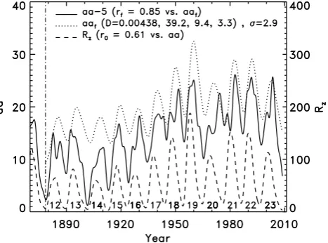
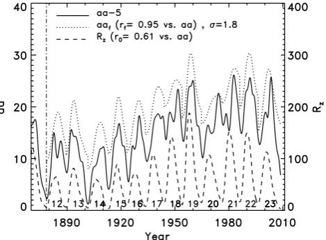
(=24 months) is the full width at half maximum (Hathaway et al., 2002). For comparison with the results of individual cycles, we employ the data from the onset of Cycle 12 (Au-gust 1878) to the end of Cycle 23 (Au(Au-gust 2008), as shown in Fig. 1:aa−5 (solid line, shifted downward by 5 for clarity) andRz(dashed) to the right of the vertical dash-dotted line. The correlation coefficient betweenaaandRzisr0=0.61 – about only one-third (r02=37.2 %) of the variation inaacan be explained by a linear correlation.
2.1 The integral response model ofaatoRz
Generally, the outputO(t )of a system will depend not only on the present inputI (t ), but also on past values. Approx-imately, O(t )is a weighted sum of the previous values of
I (t0), with the weights given by a response functionh(t−t0),
O(t )=
Z t
−∞
I (t0)h(t−t0)dt0. (2)
1ftp://ftp.ngdc.noaa.gov/STP/SOLAR
DATA/RELATED-INDICES/AA INDEX/
2http://www.ngdc.noaa.gov/stp/SOLAR/ftpsunspot-number.
Fig. 1. Monthly meanaa−5 (solid) andRz (dashed) smoothed with a 24-month Gaussian filter. The dotted line shows the recon-structedaa series (aaf) from August 1878 through August 2008 (Cycles 12–23) by Model (7). The correlation coefficients ofaa withRzandaafarer0=0.61 andrf=0.85, respectively.
In this study, the output isaaand the input isRz. Now, we determine the explicit expression of Eq. (2). Suppose that at timet=t0there is an input from solar activity, which is approximately represented byRz(t0), and that this input gen-erates an output of geomagnetic activity linearly correlated withRz(t0),
aa0(t0)=D(Rz(t0)+R0), (3)
whereD andR0 are constants, the prime onaa represents the part ofaathat is generated byRz(t0).
This activity then undergoes a decay process according to timet(due to variable current systems etc),
−1aa0∝aa01t, or ∂aa 0
∂t = −
1
τaa
0, (4)
whereτ indicates the decay time scale. Its solution is
aa0(t )=e−(t−t0)/τaa0(t0), (5) whereaa0(t0)is the integral constant att=t0, which has been already assumed to be a linear function ofRz(t0)at the initial timet=t0(Eq. 3). So that,
aa0(t )=D(Rz(t0)+R0)e−(t−t 0)/τ
. (6)
This equation means that a solar activity (Rz(t0)) at timet0 will generate a series of geomagnetic activities (aa0(t )) in the subsequent times (t > t0) according to an exponential decay factor (e−(t−t0)/τ). In other words, the geomagnetic activity at timetis generated by all the solar activities before timet, i.e., the summation of Eq. (6),
aa(t )=P
aa0(t )+aa0
=DRtt0=−∞[Rz(t0)+R0]e−(t−t 0
)/τdt0+aa 0 =DPt
t0=t0[Rz(t0)+R0]e−(t−t 0)/τ
+aa0.
(7)
In this expression, the input is the solar activity (I (t0)∝
Rz(t0)), the output is the geomagnetic activity (O(t )∝ aa(t )), and the response functionh(t−t0)∝e−(t−t0)/τ. The summation is taken over from the starting time (t0) of the series to timet.
The meanings of the parameters are as follows: (i) D
is called “Dynamic response factor”, representing the ini-tial generation efficiency of geomagnetic activity∂aai/∂Rz; (ii)τ is called “response time scale” ofaatoRz, represent-ing that a solar activity may generate a series of geomagnetic activities in the subsequent time period of aboutτ (months); (iii)aa0is a constant, representing the geomagnetic activity generated by earlier solar activities (see Sects. 3.1 and 4.2), and (iv)R0represents that some weak solar activities (mag-netic fields), which should be but have not been seen in the form of sunspots (the sunspots or dark pores are too small to be seen), may also generate geomagnetic activities. Penn and Livingston (2006) pointed out that the magnetic field has a threshold of 1500 Gauss, below which no dark pores formed, which represents a real physical limit for the formation of a dark spot (either a pore or a sunspot) on the solar photo-sphere. Weak magnetic fields may be insufficient to form sunspots, but can generate geomagnetic activities. The value ofR0just reflects the effect of these weak fields.
2.2 Four-parameter model
Firstly, we use model (7) to fit theaaseries from the onset of Cycle 12 through the end of Cycle 23. The four parameters by a least-squares-fit are
D =0.00438±0.00004, τ =39.2±0.4(month), aa0=9.4±0.2,
R0 =3.3±1.6,
(8)
where±represents the standard deviation.
Using these parameters and Model (7), theaaseries can be reconstructed, as shown in Fig. 1 (aaf, dotted line). It is seen thataafwell reflects the profile ofaa, the time delay ofaato Rz, and the increase inaaor the baseline (theaaminimum of geomagnetic cycle, or simply theaaminimum,aamin) over the twentieth century. The standard deviation of the recon-struction isσ=2.9. The correlation coefficient betweenaa
and the reconstructed series (aaf) isrf=0.85, much higher than the original value (r0=0.61) betweenaaandRz. This means that about two-thirds (rf2=72.3 %) of the variation inaacan be explained by Model (7), much higher than that (r02=37.2 %) for a linear correlation.
One may argue that, if considering the time delay ofaa
Fig. 2. (a) Correlation function betweenRzandaaof the lagL=
−200,−199,..., 200 (months). (b)aa−10 (solid),Rz(dashed), and the reconstructed seriesaal(dotted) from a linear fit ofaato theRzfifteen months earlier (9).
isrm=0.71 at a lag ofLm=15 (months). The best-fit equa-tion ofaa(t )againstRz(t−15)is given by
aa(t )=14.5±0.2+(0.0937±0.0022)Rz(t−15). (9)
The standard deviation of the regression equation isσ=3.6. Figure 2b showsaa−10 (solid, shifted downward by 10 for clarity),Rz (dashed), and the reconstructed seriesaal (dot-ted) from this linear relationship (Eq. 9). Even if consider-ing the lag time (Lm) ofaatoRz, the correlation coefficient (0.71) betweenaaandaalis still lower than that (rf=0.85) from Model (7) in Fig. 1. In addition, althoughaal can ap-proximately indicate theaamaxima (aamax), while the re-constructedaaminima fromaalalmost keep a constant level (from 15.0 to 14.8 in the range of [14.8, 16.0] with a rising factor of 14.8/15.0∼1.0) due to the small values of the solar minima (Rmin) and thus can not reflect the increasing trend in the baseline (aamin) ofaa. Therefore, to describe the re-lationship betweenaaandRz, model (7) is more appropriate than a simple linear function.
2.3 Three-parameter model
When using Model (7) to fit theaatime series in the above section, theR0value is small (3.3). Therefore, we neglectR0 and use the following three-parameter expression to refit the
aaseries for Cycles 12–23,
aa(t )=DRtt0=−∞Rz(t0)e−(t−t 0
)/τdt0+aa 0 =DPt
t0=t0Rz(t0)e−(t−t 0)/τ
+aa0.
[image:4.595.51.283.60.244.2](10)
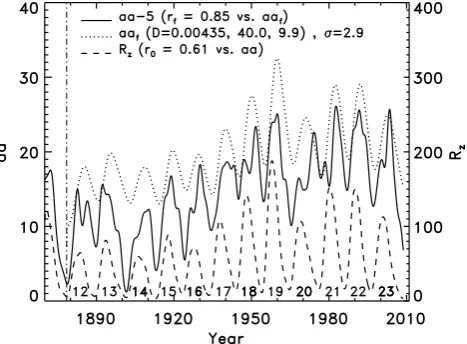
Fig. 3. Similar to Fig. 1 but using three-parameter Model (10). The correlation coefficient ofaawith the reconstructed seriesaafis also rf=0.85.
The reconstructedaaseries (aaf, dotted) is shown in Fig. 3. The three parameters based on this model,
D =0.00435±0.00004, τ =40.0±0.4(month), aa0=9.9±0.1,
(11)
have no significant changes compared with those for the four-parameter Model (8). The standard deviation of the recon-struction keeps the same level, σ=2.9. As the R0 value in Eq. (8) is very small (3.3) and the correlation coefficient between aa and the reconstructed series aaf in this case (rf=0.85) is equal to that in the case for four-parameter model in Fig. 1, the effect of three-parameter Model (10) is equivalent to that of four-parameter Model (7). Therefore, we will use the three-parameter Model (10) in the following sections.
3 Explanations for some correlations ofaawithRz
It is seen in Fig. 3 that the reconstructed series (aaf) gen-erally reflects the profile ofaa, the time delay ofaatoRz, and the increase inaaover the twentieth century. Therefore, Model (10) well represents the response of geomagnetic to solar activity, and can naturally explain in part the relation-ship betweenaaandRz.
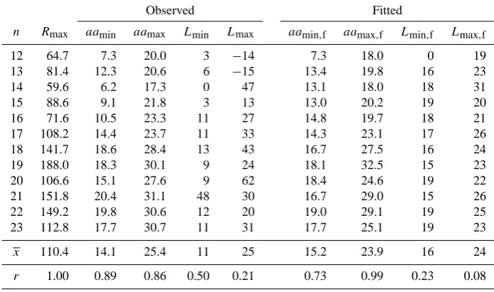
For convenience, Table 1 lists the maximum amplitude of sunspot cycle (Rmax), the preceding aa minimum (aamin), theaamaximum of geomagnetic cycle (aamax), the lag times of aa to Rz at solar minimum (Lmin) and at solar maxi-mum (Lmax), and the corresponding values (aamin,f,aamax,f, Lmin,f, Lmax,f) from the reconstructed seriesaaf in Fig. 3. The last two rows in Table 1 indicate the averages of these values and the correlation coefficients of these values with
[image:4.595.312.546.63.235.2]Table 1. Geomagnetic minimum (aamin), maximumaa(aamax), lag times ofaatoRzat minimum (Lmin) and at maximum (Lmax) for Cyclesn=12–23, and the corresponding values (aamin,f,aamax,f,Lmin,f,Lmax,f) from the reconstructed series (10). The last two rows show the averages of these values and the correlation coefficients (r) of these values with the maximum amplitude (Rmax) of sunspot cycle.
Observed Fitted
n Rmax aamin aamax Lmin Lmax aamin,f aamax,f Lmin,f Lmax,f
12 64.7 7.3 20.0 3 −14 7.3 18.0 0 19
13 81.4 12.3 20.6 6 −15 13.4 19.8 16 23
14 59.6 6.2 17.3 0 47 13.1 18.0 18 31
15 88.6 9.1 21.8 3 13 13.0 20.2 19 20
16 71.6 10.5 23.3 11 27 14.8 19.7 18 21
17 108.2 14.4 23.7 11 33 14.3 23.1 17 26
18 141.7 18.6 28.4 13 43 16.7 27.5 16 24
19 188.0 18.3 30.1 9 24 18.1 32.5 15 23
20 106.6 15.1 27.6 9 62 18.4 24.6 19 22
21 151.8 20.4 31.1 48 30 16.7 29.0 15 26
22 149.2 19.8 30.6 12 20 19.0 29.1 19 25
23 112.8 17.7 30.7 11 31 17.7 25.1 19 23
x 110.4 14.1 25.4 11 25 15.2 23.9 16 24
r 1.00 0.89 0.86 0.50 0.21 0.73 0.99 0.23 0.08
3.1 The increase inaaover the twentieth century
[image:5.595.309.546.351.522.2]It is well known that, in the twentieth century, there has been a significant increase in theaaindex (and its baseline), the reason for which, however, is unknown (Feynman and Crooker, 1978; Clilverd et al., 1998; Demetrescu and Do-brica, 2008; Lukianova et al., 2009).
Figure 4a shows the values ofaamin(solid),aamin,f (dot-ted) andRmax(dashed). It is clearly seen thataamin,fis well correlated withaamin(r=0.82) and well reflects the increas-ing trend inaamin(with rising factors of 17.7/7.4 vs. 17.7/7.3 ∼2.4). Both values (aamin,aamin,f) are well correlated with Rmax(r=0.89, 0.73).
Figure 4b shows the values ofaamax(solid),aamax,f (dot-ted) andRmax (dashed). It can also be seen thataamax,fis highly correlated withaamax(r=0.91) and well reflects the increasing trend inaamax(with rising factors of 25.1/18.0∼ 1.4 vs. 30.7/20.0∼1.5). The correlation coefficients of these two values (aamax, aamax,f) with Rmax are also very high (r=0.86, 0.99).
In Model (10), theaaindex is viewed as the total contri-butions from all the solar activities (Rz) at the present and in the past times. Therefore, the increasing trends inaa,aamax andaamin(baseline) are caused by the increasing trend inRz (Fig. 3). This confirms the suggestions that the change inaa
is caused by an increase in solar magnetic activity over the last century (Lockwood et al., 1999), and that the increasing trend in magnetic storm is most likely caused by solar ac-tivity (Clilverd et al., 1998). As the value ofaaminand its increasing trend can be well reconstructed by Model (10)
to-Fig. 4. The observed (a) geomagnetic minimum (aamin), (b) maxi-mumaa(aamax), (c) lag times ofaatoRzat solar minimum (Lmin) and (d) at maximum (Lmax) for Cyclesn=12–23 are shown by solid lines, and the corresponding values (aamin,f,aamax,f,Lmin,f, Lmax,f) from the reconstructed series (Eq. 10) are shown by dotted lines. The dashed lines in (a) and (b) show the maximum amplitude (Rmax) of sunspot cycle for comparison. The correlation coeffi-cients ofaaminwithaamin,fandRmaxarer=0.82 and 0.89, re-spectively. The correlation coefficients ofaamaxwithaamax,fand Rmaxarer=0.91 and 0.86, respectively.
3.2 The longer lag times of aa to Rz at solar maxima than at minima
Theaaindex tends to lag behindRzabout 2–3 years around a solar maximum (Wang et al., 2000; Echer et al., 2004), and about 1 year around a solar minimum (Legrand and Simon, 1981; Wilson, 1990; Wang and Sheeley, 2009).
The lag times ofLmin(solid) andLmin,f(dotted) are shown in Fig. 4c, and those ofLmax(solid) andLmax,f(dotted) are shown in Fig. 4d. It is seen that the average lag time at solar minima from the reconstructed series (Lmin,f=16) is near to the observed one (Lmin=11), and that the average lag time at solar maxima from the reconstructed series (Lmax,f=24) is close to the observed one (Lmax=25). In addition, the recon-structed series can also indicate the smaller average lag time at solar minima than at solar maxima (16<24 vs. 11<25). The weak correlations between the fitted values (Lmin,f or Lmax,f) and the observed values (Lmin or Lmax) reflect the fact thataa has several solar sources (solar flares, coronal mass ejections and solar winds etc.), and that these sources peak at different times relative toRzfor each cycle and gen-erate the geomagnetic activities with different lag times (see Discussions).
At a solar maximum, a part ofaais contributed from the solar activities (Rz) during the rising phase of the current cycle, which are weaker than the maximum value (Rmax). These smaller values ofRz lead theaa index not to reach its maximum at the same time ofRmax. After the timing of Rmax, a part ofaais contributed from the values ofRzaround the maximum (Rmax), which make theaaindex larger than that it should have been. So theaaindex reaches its maxi-mum at a time later than the timing ofRmax.
At a solar minimum, a part ofaais contributed from the solar activities (Rz) during the declining phase of the preced-ing cycle, which are stronger than the minimum value (Rmin). These larger values ofRzlead theaaindex not to reach its minimum at the same time ofRmin. After the timing ofRmin, a part ofaais contributed from the values ofRzaround the minimum (Rmin), which make theaaindex smaller than that it should have been. So theaaindex reaches its minimum at a time later than the timing ofRmin.
Because the stronger the previousRzvalues, the more they contribute to the subsequent aa values, and the longer the lag time ofaatoRz (10). The values ofRz around a solar maximum are much larger than those around the preceding minimum (andRzchanges more slowly during the declining phase near the minimum than near the maximum). There-fore, the lag times of aa to Rz near solar maxima (about two years) are longer than those near solar minima (about one year). While the linear relationship betweenaaandRz (Fig. 2) can not indicate the longer lag times ofaatoRzat solar maxima and the shorter lag times at solar minima. The sharp increase in lag time in cycle 14 (Fig. 4d) is mainly due to the higher maxima in Cycles 12–13 than that in Cycle 14.
3.3 The stronger correlations betweenaaandRzat ris-ing phases than at declinris-ing phases
According to Model (10), aa(t )at time t comes from the total contributions ofRz(t−1t )at various1t with a decay factor ofe−1t /τ. The longer the time interval ofRzpreceding aa, the less its contribution.
During the rising phase of a solar cycle, the aavalue is contributed from two parts ofRz: one is that during the same rising phase, and another is that during the previous declining phase (for simplicity, we neglect the less contributions from the even earlier data). The former varies approximately lin-early with time in an ascending way and has a linear response toaathat makes the correlation ofaawithRzpositive. The latter has a longer time delay1t and so contributes less to
aathan the former. Thus, the correlation betweenaaandRz at the rising phase of a solar cycle is strong (Du, 2011b).
During the declining phase of a solar cycle, there are also two parts ofRzthat contribute toaa: one is that during the same declining phase, and another is that during the preced-ing rispreced-ing phase. The former varies approximately linearly with time in a descending way and has a roughly linear re-sponse toaathat makes the correlation ofaawithRz posi-tive. However, the latter varies with time in an opposite as-cending way which contributes a negative correlation. Be-cause the values ofRz around a solar maximum are much larger than those around a solar minimum, the contribution of the negative correlation around the solar maximum is larger than that around the solar minimum. Thus, the correlation betweenaaandRzat the declining phase of a solar cycle is weak (Du, 2011b).
3.4 The decreasing trend in the correlation betweenaa andRz
The decreasing trend in the correlation betweenaaandRz over time is due to the increasing trend in Rz (solar mag-netic activity) over the last century (Fig. 3). The values ofRz around solar minima have no significant changes from Cy-cles 12 to 23, so there are no significant variations in the cor-relations at rising phases according to Eq. (10) and Sect. 3.3. However, the increasing trend in the values ofRzaround so-lar maxima (Rmaxin Fig. 4b) contributes increasing negative correlations ofaawithRzat the following declining phases. This leads to a descending trend in the correlations at declin-ing phases, which finally makes the correlation ofaa with
Rz decease for each cycle or for a given time window (Du, 2011b).
3.5 The increasing trend in the lag time ofaatoRz
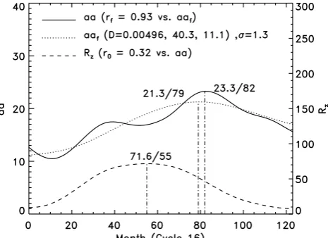
Fig. 5. Results for Cycle 16 (from April 1923 to July 1933),aa (solid),Rz(dashed), and the reconstructed seriesaaf(dotted) from Model (10). The correlation coefficients ofaawithRzandaafare r0=0.32 andrf=0.93, respectively. The peak sizes/time intervals (in months) of these peaks from the minimum are also labelled.
lag time ofaatoRz. So, the increasing trend inRz around solar maxima produces an increasing trend in the lag time of
aatoRzduring the declining phases (besides the decreasing correlation ofaawithRz).
3.6 The turning point of the correlation of aawith Rz around Cycle 19
The Rz values show a roughly increasing trend from Cy-cles 12 to 19 and a roughly declining trend since Cycle 19 (Fig. 3). This is the reasons for the decreasing trend in the correlation betweenaaandRzand the increasing lag time of aatoRzbefore Cycle 19 (Du, 2011b). These trends changed since Cycle 19 (around 1958).
4 The results for modelling each cycle of 12–23
In this section, Model (10) is applied to each Cycle of 12– 23. Considering that the values ofRz around a solar mini-mum are small and generate less geomagnetic activities than during other times, and that the activities before the solar minimum will undergo longer decay times, we take the start-ing time in the summation of Model (10) as the timstart-ing of the previous solar minimum (t0).
4.1 For an individual Cycle 16
Firstly, we apply Model (10) to an arbitrary solar Cycle 16 as an example. Figure 5 shows the time series ofaa(solid),Rz (dashed) for Cycle 16 (from April 1923 to July 1933), and the reconstructed series (aaf, dotted).
[image:7.595.51.284.62.231.2]It is seen from Fig. 5 that the reconstructed series (aaf) well reflects the profile ofaa and the time delay ofaamax
Table 2. Fitted parameters ofD, τ andaa0, and the correlation coefficients ofaawithRz(r0) andaaf(rf) for Cyclesn=12–23.
n t0 103D τ aa0 r0 rf 12 Jul 1878 7.10 24.0 9.4 0.56 0.83 13 May 1889 76.26 1.3 9.9 0.90 0.90 14 Aug 1901 6.62 27.6 8.0 0.55 0.92 15 Nov 1912 10.59 12.8 10.8 0.84 0.96 16 Apr 1923 4.96 40.3 11.1 0.32 0.93 17 Jul 1933 2.67 58.0 14.6 0.30 0.99 18 Dec 1943 1.20 53.2 19.9 0.17 0.70 19 Jan 1954 6.89 10.1 17.6 0.88 0.98 20 Sep 1964 1.02 137.0 16.6 −0.18 0.83 21 Feb 1976 1.35 58.5 20.6 −0.00 0.71 22 Jan 1986 5.17 15.3 19.5 0.76 0.96 23 Apr 1996 6.82 17.2 15.1 0.65 0.84
x 10.88 37.9 14.4 0.48 0.88
(23.3) toRmax (71.6): 79−55=24 vs. 82−55=27. The three parameters in Model (10) for Cycle 16 areD=4.96× 10⁻³,τ=40.3 (months) andaa0=11.1. The correlation co-efficient ofaawithaaf(rf=0.93) is much higher than that (r0=0.32) ofaawithRz. Besides, these results are not sen-sitive to the accurate definition of the timings of solar minima – the results remain nearly the same even if the starting time (t0) shifts a few months forward or backward.
4.2 The fitted parameters for Cycles 12–23
For each Cycle ofn=12–16, we use Model (10) to fit the
aaindex as done in the previous section. The results for all individual Cycles ofn=12–16 are shown in Fig. 10. The three parameters are listed in Table 2 and shown in Fig. 6.
It should be noted in Fig. 6a that the parametersD(solid) andτ (dotted) tend to vary in an opposite trend:Dincreases whileτ decreases, and vice versa. The correlation coefficient between them isr= −0.41 (or−0.87 if not considering the two outliers of Cycles 13 and 20). It represents the fact that the faster the energy transfer from solar activity to geomag-netic activity (via solar winds, for example) in a solar cycle, the less time the energy transfer needs. The averageDand
τ areD=10.88×10⁻³andτ=37.9 (months), respectively, implying that a solar activity will affects the geomagnetic activity in the subsequent time period of about 38 months (3 years) on average.
[image:7.595.310.542.97.271.2]Fig. 6. Parameters for Cyclesn=12–23: (a) forD(solid) andτ (dotted); (b) foraa0−5 (solid),aamin(dotted), andRmax(dashed). (c) The correlation coefficient ofaawithRz(r0, solid) and that of aawithaaf(rf, dotted). The correlations ofDwithτ,aa0, andr0 arer= −0.41,−0.40, and 0.48, respectively. The correlations of aa0withaaminandRmaxarer=0.95 and 0.89, respectively.
(aa0=14.4) is close to the averageaamin (aamin=14.1). The value ofaa0well reflects the level of and variation in aamin. These facts imply that, besides theRz values in the current cycle, theRzvalues in the previous cycles also gener-ate geomagnetic activities in the current cycle, and thataa0, likeaamin, is generated by the earlierRzvalues.
Figure 6c shows the correlation coefficient ofaawithRz (r0, solid) and that ofaawithaaf(rf, dotted) for each Cy-cle ofn=12–16 (Table 1). The average rf (rf=0.88) is much higher than the average r0 (r0=0.48). Therefore, Model (10) reflects the relationship between solar and geo-magnetic activities in a more reliable way than using a simple linear function.
The correlation coefficients ofr0 withD and τ are r= 0.48 (or 0.85 if not considering Cycles 13 and 20) and−0.91, respectively. Therefore,Dreflects the linear correlation and
τ reflects the nonlinear correlation ofaawithRz. Besides, τ is well correlated withLmax(0.70), and thusτ is related to the time delay ofaamaxtoRmax.
4.3 The reconstructedaaseries for Cycles 12–23
Combing the results of Cycles 12–23 in the above section, theaaseries from Cycles 12 through 23 can be reconstructed (aaf), as shown in Fig. 7 (dotted line).
The standard deviation of the reconstruction isσ=1.8. The correlation coefficient of aa (solid, shifted downward by 5 for clarity) withaaf(rf=0.95) is higher than the previ-ous value (0.85 in Fig. 1), and much higher than that ofaa
withRz(r0=0.61). This means that aboutrf2=90.3 % of
the variation inaacan be explained by Model (10).
Fig. 7. Time series ofaa−5 (solid) andRz(dashed) since January 1870. The dotted line shows the reconstructedaaseries (aaf) from each Cycle of 12–23 by Model (10). The correlation coefficients of aawithRzandaafarer0=0.61 andrf=0.95, respectively.
4.4 Correlations for even- and odd-numbered cycles
An even-numbered cycle is preferentially paired with the following odd-numbered one (Wilson, 1988), constituting a Hale cycle of even-odd cycle pairs: an odd-numbered cycle tends to be stronger than the previous even-numbered one, the so-called G–O rule (Gnevyshev and Ohl, 1948; Wilson, 1988). This rule is also applicable to parameterD: an odd-numbered cycle tends to have a largerDthan the previous even-numbered one (Table 2), with only one exception of the E-O pair of Cycles 16–17. A similar rule is also applicable to parameterτ: an odd-numbered cycle tends to have a shorter
τ than the previous even-numbered one (Table 2), with only two exceptions of the E-O pairs of 16–17 and 22–23.
The solar maximum (Rmax) is positively correlated withτ of the previous cycle (r=0.68, or 0.82 if not considering Cy-cle 20), and reversely correlated withDof the previous cycle (r= −0.57, or−0.93 if not considering Cycle 13). These can explain the following phenomena.
[image:8.595.50.285.62.232.2]Table 3. Parameters for Hale cycles (H).
H n RH 103DH τH 7 12–13 73.1 41.68 12 8 14–15 74.1 8.61 21 9 16–17 89.9 3.82 49 10 18–19 164.9 4.01 32 11 20–21 129.2 1.19 98 12 22–23 131.0 6.00 16
4.5 Correlations for Hale cycles
The above correlations can also explain the variation in the correlation ofaawithRzfor the Hale cycles. The even-odd cycle pairs can be numbered as the Hale cycles (H) such thatH=7 for Cyclesn=12-13,H=8 forn=14-15,···,
H=12 forn=22-23. The averages ofRz,Dandτ forH -cycles are listed in Table 3 such thatRH(7)= [Rmax(12)+ Rmax(13)]/2, etc.
It is seen in Table 3 that an even-numberedH-cycle tends to be stronger than the previous odd-numbered one. Since
H=8, an even-numberedH-cycle tends to have a larger
D and a shorterτ than the neighboring odd-numbered H -cycle. Therefore, an even-numberedH-cycle tends to have a stronger correlation and a shorter lag time ofaatoRzthan the neighboring odd-numberedH-cycle (Du, 2011b).
5 Discussions and conclusions
It has been known that there are two main solar sources of geomagnetic activity (Legrand and Simon, 1981, 1989; Gon-zalez and Tsurutani, 1987; GonGon-zalez et al., 2004; Venkatesan et al., 1991; Echer et al., 2004; Tsurutani et al., 2006). One source (coronal mass ejections or CMEs) has a frequency of occurrence that is in phase with the sunspot cycle while the second source (high-speed solar wind streams) is out of phase with the sunspot cycle. Feynman (1982), through an-alyzing the relationship between the annualaaandRzfrom 1869 to 1975, decomposedaainto two equally strong peri-odic components: one (the “short lived” R component) as-sociated with solar flares, prominence eruptions, and CMEs which follows the solar activity cycle and a second compo-nent (the “slowly varying” I compocompo-nent) associated with re-current high speed solar wind streams which is out of phase with the solar activity cycle (Hathaway and Wilson, 2006). Legrand and Simon (1989) classified the geomagnetic ac-tivity (aa index) in four classes related to solar activity: (1) the magnetic quiet activity due to slow solar wind flowing around the magnetosphere, (2) the recurrent activity related to high wind speed solar wind, (3) the fluctuating activity re-lated to fluctuating solar wind and (4) the shock activity due to shock events (CMEs).
A primary physical mechanism for energy transfer from the solar wind to the magnetosphere is magnetic reconnec-tion between the interplanetary magnetic field (IMF) and the Earth’s magnetic field (Dungey, 1961; Gonzalez et al., 1994; Tsurutani et al., 1995; Zhang et al., 2007). The intensity and the orientation of the solar dipole is the source of the recur-rent storms, while the size and the shape of the neutral sheet are the sources both of the quiet days and of the fluctuating activity (Simon and Legrand, 1989). However, there are no accurate expressions to clearly describe the relationship be-tween the solar and geomagnetic activities.
The magnetic field is a crucial quantity to determine the state of the solar atmosphere and plays a key role in the for-mation and dynamics of solar activity. Sunspots (Rz) rep-resent one of the most obvious manifestations of local mag-netic fields on the Sun. The solar activity affects the geomag-netic activity in various complex processes from the Sun to the Earth, involved in the solar – interplanetary – magneto-spheric – ionomagneto-spheric couplings (Tsurutani et al., 2006). The
aageomagnetic index integrates all the effects on magneto-sphere of several sources, such as solar flares, CMEs, and fast solar wind streams. The relationship betweenaaandRz is not a simple linear or nonlinear function, rather it is an integral response function (10).
In this study, we presented a integral response model,
aa(t )=DRtt0= −∞Rz(t
0)e−(t−t0)/τdt0+aa
0, to describe the relationship between the output (geomagnetic activity, aa) and the input (solar activity,Rz) of a (solar-terrestrial) sys-tem. In this model, the outputaa(t ) depends not only on the present inputRz(t ), but also on past values. The output is a weighted sum of previous values of the input (Eqs. 2, 10), and the weights are given by the response function,
h(t−t0)∝e−(t−t0)/τ. The earlier the input, the less it con-tributes to the output. ParameterDrepresents the “Dynamic response factor” ofaatoRz and reflects the linear correla-tion of aa withRz. Parameterτ represents the “response time scale” ofaatoRz(it needs time for the energy transfer from solar to geomagnetic activity) and reflects the nonlinear correlation ofaawithRz. Parameteraa0represents the ge-omagnetic activity generated by earlier solar activities (Rz, solar flares, CMEs, shocks, and solar winds etc.). For each solar cycle theaa0value reflects and is well correlated with the geomagnetic minimum (aamin).
For a linear relationship, the correlation coefficient be-tween theaaandRzseries (3) is only r0=0.61, implying that only aboutr02=37.2 % of the variation inaacan be ex-plained by a linear dependence. However, when using our Model (10), the correlation betweenaaand the reconstructed series (aaf) for the overall data (Fig. 3) is much higher (rf= 0.85) than the above value, implying that aboutrf2=72.3 % of the variation inaacan be explained by Model (10). If this model is applied to each solar cycle, the correlation will be even higher (rf=0.95), implying that aboutrf2=90.3 % of
Fig. 8. (a) Monthly mean of integrated daily CME linear speedV−
200 (solid, shifted downward by 200 for clarity) andRz(dashed) smoothed with a 24-month Gaussian filter. The dotted line shows the reconstructed series (Vf) from January 1998 to September 2008 by Model (10). The correlation coefficients ofV withRzandVf arer0=0.936 andrf=0.993, respectively. The lag time ofV to Rz(at maximum) isL1=16 (months). (b) Similar results for the relationship betweenaa (solid) andV (dashed). The correlation coefficients ofaawithV and the reconstructed seriesaafarer0= 0.79 andrf=0.80, respectively. The lag time ofaatoV isL2= 15 (months). (c) Similar results for the relationship betweenaa (solid) andRz (dashed). The correlation coefficients ofaa with Rz and the reconstructed seriesaaf are r0=0.65 and rf=0.84, respectively. The lag time ofaatoRzisL=31 (months). Other numbers indicate the fitted parameters (D,τ,y0) andσ.
This model can naturally explain in part the time delay of
aatoRzand the following phenomena.
1. The significant increase in theaaindex over the twen-tieth century (Feynman and Crooker, 1978; Clilverd et al., 1998; Demetrescu and Dobrica, 2008; Lukianova et al., 2009), in either the cycle-averaged level or the base-line (Figs. 3, 4a, b and 6b).
2. The longer lag times ofaatoRzat solar maxima than at solar minima (Legrand and Simon, 1981; Wilson, 1990; Wang et al., 2000; Echer et al., 2004; Wang and Sheeley, 2009).
3. The stronger correlations betweenaaandRzat rising phases than at declining phases (Du, 2011b).
4. The decreasing trend in the correlation betweenaaand
Rz over time (Borello-Filisetti et al., 1992; Kishcha et al., 1999; Du, 2011b).
5. The increasing trend in the lag time ofaatoRz over time (Du, 2011b).
6. The turning point of the correlation of aa with Rz around Cycle 19 (Du, 2011b).
Fig. 9. Similar to Fig. 8 but using the double-decay model (12). (a) The correlation coefficient ofV (solid, shifted downward by 200 for clarity) with the reconstructed seriesVf(dotted) fromRz (dashed) by Eq. (12) is nowrf=0.997. (b) The correlation co-efficient ofaa(solid, shifted downward by 3 for clarity) with the reconstructed seriesaaf (dotted) fromV (dashed) by Eq. (12) is nowrf=0.92. (c) The correlation coefficient ofaa(solid, shifted downward by 3 for clarity) with the reconstructed seriesaaf (dot-ted) fromRz(dashed) by Eq. (12) is nowrf=0.91.
7. The stronger correlations (and shorter lag times) at odd-numbered cycles than at the previous even-odd-numbered cycles (Du, 2011b).
8. The stronger correlations (and shorter lag times) at even-numbered H-cycles than at the previous odd-numberedH-cycles (Du, 2011b).
The decreasing trend in the correlation betweenaaandRz has ever been explained by the increasing occurrence of high-speed solar wind streams during the declining phase of so-lar cycle (Bame et al., 1976; Borello-Filisetti et al., 1992; Mussino et al., 1994; Tsurutani et al., 1995; Kishcha et al., 1999). However, during the declining phase of solar cycle, why does the occurrence of high-speed solar wind streams increase? In our Model (10), this trend is also due to the increasing trend in solar magnetic activity (Rz) over the last century (Sect. 3.1).
[image:10.595.50.283.61.233.2] [image:10.595.310.547.64.233.2]Fig. 10. Monthly meanaa−5 (solid, shifted downward by 5 for clarity) andRz(dashed) smoothed with a 24-month Gaussian filter, and the reconstructedaaseries (aaf, dotted) by Model (10) for each cycle ofn=12 to 23. In each plot are also shown the correlation coefficient of aawithRz(r0), that ofaawithaaf (rf), and the three parameters ofD,τandaa0.
solar flares) are produced soon or close in time to the for-mation of sunspots (Rz). These events affect the geomag-netic fields (aa) in a more linear manner. Some of other events (solar winds) are produced later than the formation of sunspots, whose effect onaais in a more nonlinear man-ner. These activities may be produced in different (nonlinear) processes more or less similar to Eq. (10), and play a role of mid-processes from the solar magnetic activity (Rz) through coronal magnetic activity to geomagnetic activity (aa). This may be the reasons why solar winds are later thanRz and occur often during declining phases, and why there are often more peaks in theaa index. A similar process is also ap-plicable to the relationships betweenaaand these activities (solar flares, CMEs and solar winds). The effects of these processes are all integrated in Model (10).
As an example, we study the correlations of CME with so-lar activity (Rz) and geomagnetic activity (aa). Figure 8a shows the monthly mean of integrated daily CME linear
speed3V (solid, shifted downward by 200 for clarity) andRz (dashed) smoothed with a 24-month Gaussian filter (Eq. 1). The dotted line shows the reconstructed series (Vf) from Jan-uary 1998 to September 2008 based on Model (10). One can see that V lags behind Rz about L1=16 (months) at the solar maximum and that the correlation coefficient ofV
with the reconstructed seriesVf(rf=0.993) is higher than that (r0=0.936) ofV withRz, meaning that about 98.6 % (87.6 %) of the variation inV can be explained by this model (linear dependence).
Figure 8b shows the relationship betweenaa (solid) and
V (dashed). One can also see thataalags behindV about
L2=15 (months) and that the correlation coefficient ofaa with the reconstructed seriesaaf (rf=0.80) by Model (10) is higher than that (r0=0.79) ofaawithV. Figure 8c shows the relationship between aa (solid) and Rz (dashed). The correlation coefficient ofaawith the reconstructed seriesaaf
(rf=0.84) by Model (10) is higher than that (r0=0.65) of aawithRz. It should be pointed out that the lag time ofaato Rz(L=31 months) is longer than the lag times of bothV to Rz(L1) andaatoV (L2), and equal toL1+L2. This fact just reflects the energy transfer from solar activity (Rz) through a mid-process (CME in this case) to geomagnetic activity (aa). Similar conclusions may also hold for other solar activities (solar flares and solar winds etc) that have different lag times relative toRzand that generate geomagnetic activities with different lag times relative to these activities.
AsRz andaa are only rough estimates of solar and ge-omagnetic activities, respectively, the gege-omagnetic activity (aa) is only partially predictable by theRzindex. Besides, there are two peaks in eitheraaor CME-related storms, one near the peak inRz and another a few years later (Gonza-lez and Tsurutani, 1987; Gonza(Gonza-lez et al., 1994, 2004; Tsu-rutani et al., 2006), while there is usually only one peak in Model (10) for a solar cycle. So this model can only de-scribe the main profile ofaaand can not predict its fine struc-tures. The fine structures are related to short-time variations in the sources ofaa(CMEs, solar winds and coronal holes etc.) and solar magnetic fields (in either solar surface or so-lar corona) as well. To improve the relationship between the outputy(t )and inputx(t ), the following double-decay model can be used,
y(t )=Rt
t0=−∞x(t0)
h
D1e−(t−t 0
)/τ1+D 2e−(t−t
0
)/τ2idt0+y 0
=Pt t0=t0x(t0)
h
D1e−(t−t 0
)/τ1+D 2e−(t−t
0 )/τ2i+y
0. (12)
The results based on Model (12) using the data of Fig. 8 are shown in Fig. 9.
It is seen in Fig. 9a that the correlation coefficient ofV
(solid, shifted downward by 200 for clarity) with the recon-structed seriesVf(dotted) fromRz(dashed) by Model (12) is now rf=0.997, slightly higher than that (0.993) of V with the reconstructed series based on Model (10) in Fig. 8a. In Fig. 9b, the correlation coefficient ofaa (solid, shifted downward by 3 for clarity) with the reconstructed series
aaf (dotted) fromV (dashed) by Eq. (12) is nowrf=0.92, higher than that (0.80) ofaawith the reconstructed series by Model (10) in Fig. 8b. Figure 9c shows that the correlation coefficient (rf=0.91) ofaa (solid, shifted downward by 3 for clarity) with the reconstructed seriesaaf (dotted) from Rz(dashed) by Eq. (12) is higher than that (0.84) ofaawith the reconstructed series by Model (10) in Fig. 8c.
The main profile of aa can be well predicted from the
Rz series by Model (10). Even if using another more complex function, such as a geometric function ofaa(t )=
DRt
t0= −∞R
γ
z(t0)e−(t−t 0)/τ
dt0+aa0 with an additional pa-rameterγ, there will be no significant improvement in the correlation (rfincreases from 0.85 to only 0.86). Therefore, the relationship betweenaaandRzis mainly due to the in-tegral response function. The relationship can be improved by the double-decay model (12). If considering two differ-ent lag times ofy tox in Eq. (12), the result might be
fur-ther improved. The remainder might be explained by ofur-ther activities, such as nonlinear Alfv´en waves, cosmic rays (Na-gashima et al., 1991), and the interaction (Corotating Inter-action Regions or CIRs) of fast with slow solar wind streams (Simon and Legrand, 1986; Richardson and Cane, 2002; Tsu-rutani et al., 2006), etc.
The main points of this paper may be summarized as fol-lows,
1. An integral response model is proposed to de-scribe the relationship between the geomagnetic index (aa) and sunspot number (Rz): aa(t ) = DRtt0=
−∞Rz(t
0)e−(t−t0)/τdt0+aa
0. Parameters D and τreflect the linear and nonlinear correlations ofaawith
Rz, respectively. Parameteraa0represents the geomag-netic activity generated by earlier solar activities. 2. For all data from Cycles 12 through 23, the correlation
coefficient ofaawith the reconstructed series based on this model (rf=0.85) is much higher than the linear cor-relation coefficient (r0=0.61) ofaawithRz.
3. If this model is applied to each solar cycle, the corre-lation coefficient ofaawith the reconstructed series is higher (rf=0.95). Theaa0 values reflects and is well correlated with theaaminimum of solar cycle. 4. This model can naturally explain in part some
phenom-ena related to the correlation ofaawithRz, the lag time ofaatoRz, and their temporal variations.
Acknowledgements. The authors are grateful to the anonymous ref-erees for suggestive and helpful comments. This work is supported by Chinese Academy of Sciences through grant YYYJ-1110, the National Natural Science Foundation of China (NSFC) through grants 10973020, 40890161 and 10921303, and National Basic Re-search Program of China through grants 2011CB811406.
Topical Editor P. Drobinski thanks two anonymous referees for their help in evaluating this paper.
References
Bachmann, K. T. and White, O. R.: Observations of hysteresis in solar cycle variations among seven solar activity indicators, Sol. Phys., 150, 347–357, 1994.
Bame, S. J., Asbridge, J. R., Feldman, W. C., and Gosling, J. T.: So-lar cycle evolution of high-speed soSo-lar wind streams, Astrophys. J., 207, 977–980, 1976.
Borello-Filisetti, O., Mussino, V., Parisi, M., and Storini, M.: Long-term variations in the geomagnetic activity level. I – A connec-tion with solar activity, Ann. Geophys., 10, 668–675, 1992, http://www.ann-geophys.net/10/668/1992/.
Cameron, R. and Sch¨ussler, M.: Solar Cycle Prediction Using Pre-cursors and Flux Transport Models, Astrophys. J., 659, 801–811, 2007.
Crooker, N. U., Feynman, J., and Gosling, J. T.: On the high corre-lation between long-term averages of solar wind speed and geo-magnetic activity, J. Geophys. Res., 82, 1933–1937, 1977. Demetrescu, C. and Dobrica, V.: Signature of Hale and Gleissberg
solar cycles in the geomagnetic activity, J. Geophys. Res., 113, A02103, doi:10.1029/2007JA012570, 2008.
Du, Z. L.: The correlation between solar and geomagnetic activity – Part 1: Two-term decomposition of geomagnetic activity, Ann. Geophys., in review, 2011a.
Du, Z. L.: The correlation between solar and geomagnetic activity – Part 2: Long-term trends, Ann. Geophys., in review, 2011b. Du, Z. L. and Wang, H. N.: Is a higher correlation necessary for a
more accurate prediction? Science China (Physics, Mechanics & Astronomy), 54, 172–175, 2011.
Du, Z. L., Li, R., and Wang, H. N.: The Predictive Power of Ohl’s Precursor Method, Astron. J., 138, 1998–2001, 2009.
Dungey, J. W.: Interplanetary magnetic field and the auroral zones, Phys. Rev. Lett., 6, 47–48, 1961.
Echer, E., Gonzalez, W. D., Gonzalez, A. L. C., Echer, E., Gonza-lez, W. D., GonzaGonza-lez, A. L. C., Prestes, A., Vieira, L. E. A., dal Lago, A., Guarnieri, F. L., and Schuch, N. J.: Long-term correla-tion between solar and geomagnetic activity, J. Atmos. Sol. Terr. Phys., 66, 1019–1025, 2004.
Feynman, J.: Implications of solar cycles 19 and 20 geomagnetic activity for magnetospheric processes, Geophys. Res. Lett., 7, 971–973, 1980.
Feynman, J.: Geomagnetic and solar wind cycles, 1900–1975, J. Geophys. Res., 87, 6153–6162, 1982.
Feynman, J. and Crooker, N. U.: The solar wind at the turn of the century, Nature, 275, 626–627, 1978.
Garrett, H. B., Dessler, A. J., and Hill, T. W.: Influence of solar wind variability on geomagnetic activity, J. Geophys. Res., 79, 4603–4610, 1974.
Gnevyshev, M. N. and Ohl, A. I.: On the 22-year solar activity cycle, Astron. Z., 25, 18–20, 1948.
Gonzalez, W. D. and Tsurutani, B. T.: Criteria of interplanetary parameters causing intense magnetic storms (Dst of less than
−100 nT), Planet. Space Sci., 35, 1101–1109, 1987.
Gonzalez, W. D., Gonzalez, A. L. C., Tsurutani, B. T., Smith, E. J., and Tang, F.: Solar wind-magnetosphere coupling during intense magnetic storms (1978–1979), J. Geophys. Res., 94, 8835–8851, 1989.
Gonzalez, W. D., Joselyn, J. A., Kamide, Y., Kroehl, H. W., Ros-toker, G., Tsurutani, B. T., and Vasyliunas, V. M.: What is a geomagnetic storm?, J. Geophys. Res., 99, 5771–5792, 1994. Gonzalez, W. D., Dal Lago, A., Clua de Gonzalez, A. L., Vieira, L.
E. A., and Tsurutani, B. T.: Prediction of peak-Dst from halo CME-magnetic cloud-speed observations, J. Atmos. Sol. Terr. Phys., 66, 161–165, 2004.
Gosling, J. T. and Pizzo, V. J.: Formation and evolution of coro-tating interaction regions and their three dimensional strcture, Space Sci. Rev., 89, 21–52, 1999.
Hathaway, D. H. and Wilson, R. M.: Geomagnetic activity indicates large amplitude for sunspot cycle 24, Geophys. Res. Lett., 33, L18101, doi:10.1029/2006GL027053, 2006.
Hathaway, D. H., Wilson, R. M., and Reichmann, E. J.: Group sunspot numbers: sunspot cycle characteristics, Solar Phys., 211, 357–370, 2002.
Johnson, J. R. and Wing, S.: A solar cycle dependence of
nonlinear-ity in magnetospheric activnonlinear-ity, J. Geophys. Res., 110, A04211, doi:10.1029/2004JA010638, 2005.
Kishcha, P. V., Dmitrieva, I. V., and Obridko, V. N.: Long-term variations of the solar – geomagnetic correlation, total solar ir-radiance, and northern hemispheric temperature (1868–1997), J. Atmos. Sol. Terr. Phys., 61, 799–808, 1999.
Legrand, J. P. and Simon, P. A.: Ten cycles of solar and geomagnetic activity, Solar Phys., 70, 173–195, 1981.
Legrand, J. P. and Simon, P. A.: Solar cycle and geomagnetic ac-tivity: A review for geophysicists. I – The contributions to ge-omagnetic activity of shock waves and of the solar wind, Ann. Geophys., 7, 565–578, 1989,
http://www.ann-geophys.net/7/565/1989/.
Lockwood, M., Stamper, R., and Wild, M. N.: A doubling of the Sun’s coronal magnetic field dring the past 100 years, Nature, 399, 437–439, 1999.
Lukianova, R., Alekseev, G., and Mursula, K.: Effects of sta-tion relocasta-tion in the aa index, J. Geophys. Res., 114, A02105, doi:10.1029/2008JA013824, 2009.
Mayaud, P. N.: The aa indices: A 100-year series characterizing the magnetic activity, J. Geophys. Res., 77, 6870–6874, 1972. Moradi, H., Baldner, C., Birch, A. C., Braun, D. C., Cameron, R. H.,
Duvall Jr., T. L., Gizon, L., Haber, D., Hanasoge, S. M., Hind-man, B. W., Jackiewicz, J., Khomenko, E., Komm, R., Rajaguru, P., Rempel, M., Roth, M., Schlichenmaier, R., Schunker, H., Spruit, H. C., Strassmeier, K. G., Thompson, M. J., and Zharkov, S.: Modeling the Subsurface Structure of Sunspots, Solar Phys., 267, 1–62, 2010.
Mursula, K., Martini, D., and Karinen, A.: Did open solar magnetic field increase during the last 100 years? A reanalysis of geomag-netic activity, Solar Phys., 224, 85–94, 2004.
Mussino, V., Borello Filisetti, O., Storini, M., and Nevanlinna, H.: Long-term variations in the geomagnetic activity level Part II: Ascending phases of sunspot cycles, Ann. Geophys., 12, 1065– 1070, doi:10.1007/s00585-994-1065-5, 1994.
Nagashima, K., Fujimoto, K., and Tatsuoka, R.: Nature of solar-cycle and heliomagnetic-polarity dependence of cosmic rays, in-ferred from their correlation with heliomagnetic spherical sur-face harmonics in the period 1976–1985, Planet. Space Sci., 39, 1617–1635, 1991.
Nevanlinna, H. and Kataja, E.: An extension of the geomagnetic ac-tivity index series aa for two solar cycles (1844–1868), Geophys. Res. Lett., 20, 2703–2706, 1993.
Parker, E. N.: Interplanetary Dynamical Processes, Interscience Publishers, New York, 1963.
Penn, M. J. and Livingston, W.: Temporal Changes in Sunspot Um-bral Magnetic Fields and Temperatures, Astrophys. J., 649, L45– L48, 2006.
Prestes, A., Rigozo, N. R., Echer, E., and Vieira, L. E. A.: Spec-tral analysis of sunspot number and geomagnetic indices (1868– 2001), J. Atmos. Sol. Terr. Phys., 68, 182–190, 2006.
Richardson, I. G. and Cane, H. V.: Sources of geomagnetic activity during nearly three solar cycles (1972–2000), J. Geophys. Res., 107(A8), SSH 8-1, 1187, doi:10.1029/2001JA000504, 2002. Russell, C. T. and McPherron, R. L.: Semiannual variation of
geo-magnetic activity, J. Geophys. Res., 78, 92–108, 1973.
Sakurai, T.: Calculation of force-free magnetic field with non-constantα, Solar Phys., 69, 343–359 , 1981.
Sargent, H. H.: Recurrent geomagnetic activity - Evidence for long-lived stability in solar wind structure, J. Geophys. Res., 90, 1425–1428, 1985.
Schatten, K. H. and Pesnell, W. D.: An early solar dynamo predic-tion: Cycle 23 is approximately cycle 22, Geophys. Res. Lett., 20, 2275–2278, 1993.
Schatten, K. H., Scherrer, P. H., Svalgaard, L., and Wilcox, J. M.: Using dynamo theory to predict the sunspot number during solar cycle 21, Geophys. Res. Lett., 5, 411–414, 1978.
Schwenn, R.: Solar wind sources and their variations over the solar cycle, Space Sci. Rev., 124, 51–76, 2006.
Simon, P. A. and Legrand, J. P.: Some solar cycle phenomena re-lated to the geomagnetic activity from 1868 to 1980, Astron. As-trophys., 155, 227–236, 1986.
Simon, P. A. and Legrand, J. P.: Solar cycle and geomagnetic activ-ity: A review for geophysicists. II – The solar sources of ge-omagnetic activity and their links with sunspot cycle activity, Ann. Geophys., 7, 579–593, 1989.
Snyder, C. W., Neugebauer, M., and Rao, U. R.: The Solar Wind Ve-locity and Its Correlation with Cosmic-Ray Variations and with Solar and Geomagnetic Activity, J. Geophys. Res., 68, 6361– 6370, 1963.
Stamper, R., Lockwood, M., Wild, M. N., and Clark, T. D. G.: So-lar causes of the long-term increase in geomagnetic activity, J. Geophys. Res., 104, 28325–28342, 1999.
Svalgaard, L.: Geomagnetic activity: Dependence on solar wind parameters, in: Coronal Holes and High Speed Wind Streams, edited by: Zirker, J. B., Colorado Ass. U. Press, Boulder, p. 371, 1977.
Temmer, M., Veronig, A., and Hanslmeier, A.: Does solar flare ac-tivity lag behind sunspot acac-tivity? Solar Phys., 215, 111–126, 2003.
Tsurutani, B. T., Gonzalez, W. D., Tang, F., Akasofu, S. I., and Smith, E. J.: Origin of interplanetary southward magnetic fields responsible for major magnetic storms near solar maximum (1978–1979), J. Geophys. Res., 93, 8519–8531, 1988.
Tsurutani, B. T., Gonzalez, E. D., Gonzalez, A. L. C., Tang, F., Ar-ballo, J. K., and Okada, M.: Interplanetary origin of geomagnetic activiy in the declining phase of the solar cycle, J. Geophys. Res., 100, 21717–21733, 1995.
Tsurutani, B. T., Gonzalez, W. D., Gonzalez, A. L. C., Guarnieri, F. L., Gopalswamy, N., Grande, M., Kamide, Y., Kasahara, Y., Lu, G., Mann, I., McPherron, R., Soraas, F., and Vasyli-unas, V.: Corotating solar wind streams and recurrent geo-magnetic activity: A review, J. Geophys. Res., 111, A07S01, doi:10.1029/2005JA011273, 2006.
Tu, C. Y. and Marsch, E.: MHD structures, waves and turbulence in the solar wind: observations and theories, Space Sci. Rev., 73, 1–210, 1995.
Venkatesan, D., Ananth, A. G., Graumann, H., and Pillai, S.: Re-lationship between solar and geomagentic activity, J. Geophys. Res., 96, 9811–9813, 1991.
Wang, Y. M. and Sheeley, N. R.: Understanding the Geomagnetic Precursor of the Solar Cycle, Astrophys. J., 694, L11–L15, 2009. Wang, Y. M., Lean, J., and Sheeley, N. R.: The long-term variation of the Sun’s open magnetic flux, Geophys. Res. Lett., 27, 505– 508, 2000.
Wheatland, M. S. and Litvinenko, Y. E.: Energy balance in the flar-ing solar coronaA, Astrophys. J., 557, 332–336, 2001.
Wilson, R. M.: Bimodality and the Hale cycle, Solar Phys., 117, 269–278, 1988.
Wilson, R. M.: On the level of skill in predicting maximum sunspot number – A comparative study of single variate and bivariate precursor techniques, Solar Phys., 125, 143–155, 1990. Yan, Y. and Li, Z.: Direct Boundary Integral Formulation for Solar
Non-constant-αForce-free Magnetic Fields, Astrophys. J., 638, 1162–1168, 2006.