ORIGINAL ARTICLE
Controlling Roll Temperature
by Fluid-Solid Coupled Heat Transfer
Jing‑Feng Zou
1,2, Li‑Feng Ma
1,2, Guo‑Hua Zhang
1,2*, Zhi‑Quan Huang
1,2, Jin‑Bao Lin
1and Peng‑Tao Liu
1Abstract
Currently, when magnesium alloy sheet is rolled, the method of controlling roll temperature is simple and inaccurate. Furthermore, roll temperature has a large influence on the quality of magnesium alloy sheet; therefore, a new model using circular fluid flow control roll temperature has been designed. A fluid heat transfer structure was designed, the heat transfer process model of the fluid heating roll was simplified, and the finite difference method was used to cal‑ culate the heat transfer process. Fluent software was used to simulate the fluid‑solid coupling heat transfer, and both the trend and regularity of the temperature field in the heat transfer process were identified. The results show that the heating efficiency was much higher than traditional heating methods (when the fluid heat of the roll and tempera‑ ture distribution of the roll surface was more uniform). Moreover, there was a bigger temperature difference between the input and the output, and after using reverse flow the temperature difference decreased. The axial and circum‑ ferential temperature distributions along the sheet were uniform. Both theoretical calculation results and numerical simulation results of the heat transfer between fluid and roll were compared. The error was 1.8%–12.3%, showing that the theoretical model can both forecast and regulate the temperature of the roll (for magnesium alloy sheets) in the rolling process.
Keywords: Magnesium alloy, Fluid heating, Heat transfer model, Numerical simulation of fluid‑solid coupling
© The Author(s) 2018. This article is distributed under the terms of the Creative Commons Attribution 4.0 International License (http://creat iveco mmons .org/licen ses/by/4.0/), which permits unrestricted use, distribution, and reproduction in any medium, provided you give appropriate credit to the original author(s) and the source, provide a link to the Creative Commons license, and indicate if changes were made.
1 Introduction
Magnesium alloy sheets have low density, good thermal conductivity, high specific strength and stiffness, desir-able damping properties, and excellent electromagnetic shielding. Therefore they are widely used in the aviation, aerospace [1], automobile [2], high-speed rail, and elec-tronics industries [3]. Consequently, magnesium alloy sheets have become the most promising non-ferrous metal material in the world today [4–6]. In the rolling process of magnesium alloy sheets, the roll tempera-ture has a large influence on plate quality [7]. When the roll temperature is too low, the edges crack and surface cracking of the plate occurs. When the roll temperature is too high, the roll can become stuck [8, 9]. There is an urgent need to make an important breakthrough in the accurate control of roll temperature.
In recent years, the traditional methods for heating the roll have included the induction heating method, resist-ance wire heating method, and flame heating method [10,
11]. These traditional methods suffer from long heating times and uneven heating, therefore a new model using circular fluid flow to control roll temperature has been designed. This method heats and cools the roll using two tanks. The roll temperature can be controlled by adjust-ing the velocity and temperature of the fluid. A high pre-cision heat transfer model (between the magnesium alloy sheet and roll) has been built, and the regulation strategy of roll temperature is given, meaning the roll temperature can be controlled within a reasonable range at any time. Therefore, this study can solve the existing problems of large crown, serious wave-shapes, and stuck rolls caused by inaccurate roll temperature control. This will signifi-cantly increase the finished production rate of the mag-nesium alloy sheets.
Heat transfer in the rolling process of magnesium alloy sheet is complex [12]. It includes deformation heat, fric-tion heat, thermal radiafric-tion, convective heat transfer
Open Access
*Correspondence: [email protected]
1 Heavy Machinery Engineering Research Center of the Ministry
Education, Taiyuan University of Science and Technology, Taiyuan 030024, China
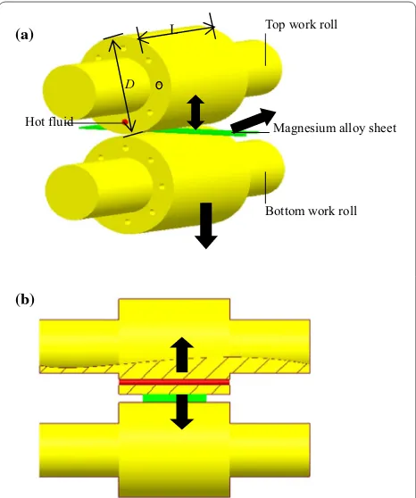
within the air between the magnesium alloy sheet and roll, and heat transfer between fluid and the roll [13–15]. These are indicated by the arrows in Figure 1. The tem-perature field in the rolling process is divided into two stages because of the complexity: single coupled heat transfer between the fluid and roll, and coupled heat transfer factors of the rolling process. The first stage is studied in this paper (the second stage will be stud-ied later), then an experiment and modifications to the model are conducted. An experimental roll (D= 320 mm,
L= 350 mm) is the chosen object to establish a fluid-solid coupled model of the fluid heating transfer roll. The roll temperature is studied for different times and velocities when fluid is heating the roll. The results are both an important and significant guide for controlling the roll temperature in the rolling process.
2 Design of the Roll Structure Using Fluid Heat Transfer
The thermostat oil holes on the roll were designed to force the fluid to flow cyclically through the oil holes, as shown in Figure 2. To prevent a problems caused by insufficient bending stiffness, the roll bending strength reduced rate (M) was less than 8% when the roll was designed. The roll bending rigidity before drilling is
EπD4
64 , the smallest roll bending rigidity after drilling is
EπD4−2nπd40−16πQs2d20
64 , the roll stiffness reduction is
E
2nπd4
0
64 −Q
πs2d2
0 4
, and the roll bending strength
reduced rate is M= (2nd 2
0+16Qs2)d02
D4 ×100%≤8%.
Here, E is the modulus of elasticity of the roll (Pa); d0 is the diameter of thermostat oil hole (m); D is the diameter of the roll (m); s is the distance between the center of the thermostat hole and cross-sectional center of the roll (m); n is half the number of thermostat oil holes (the thermostat oil hole number is even).
Q=min
k=2n−1
k=0
sin
x+π
nk
2
(k is an integer, x is a
real number and satisfies −πn ≤x≤ πn, and the Q value can be obtained by mathematical software (MATLAB).
With the roll as the research object, the diameter of the thermostat hole is d0= 0.02 m, the distance between the center of the thermostat hole and the cross-sectional center of the roll was s= 0.12 m, the number of thermo-stat oil holes was 8, and the roll bending strength reduced rate was 4.528%. This met the requirements. The two directions of the roll cross section in Figure 2 are shown in Figure 3(a) and (b). Fluid flows from oil hole 1, passed through oil holes 2‒7, then finally flowed from oil hole 8.
3 Establishment of the Analytical Model for Heat Transfer
The most accurate method for solving heat conduction is by mathematical analysis. However, the analysis can only solve the simple problem of heat conduction, whereas many of the complex thermal problems can only be obtained by numerical calculations using the finite differ-ence method [16–19].
3.1 Hypothetical Condition
(1) The model of the fluid heat transfer roll is three-dimensional. The temperature is transmitted from the inner surface of the oil hole in the radial direc-Hot fluid
Top work roll
Bottom work roll Magnesium alloy sheet L
D (a)
(b)
Figure 1 Heat transfer in the process of magnesium alloy sheet rolling
O R R F ORR F
W D H K WHD K $
$
% %
1 Y 1 Y
2 Y 2 Y
P A B P
A B
tion (the temperature difference in the circumfer-ential direction can be neglected), so the model can be simplified as two-dimensional. This means the heat transfer is along the radial and axial directions, and the roll temperature field changes with time and position. Therefore, the model of the fluid heat transfer roll was simplified to a two-dimensional unsteady heat conduction model of a hollow cylin-der.
(2) The physical property parameters of the roll and the fluid are not changed with time.
(3) The boundary conditions of fluid heat transfer, the roll inner and outer walls, and the outside are con-sidered as the third boundary condition.
3.2 Calculation of Heating Transfer Process
The temperature distribution on the hollow cylinder T(r,
t) changes with the time t and position r, the initial tem-perature distribution is T(r, 0) =T(r), r1 is the radius of the thermostat oil hole, and r2 is the closest distance from the thermostat oil hole center to the roll surface: r1= d20 =0.01 m,r2= 0.04 m, and r1 < r < r2, as shown in Figure 3.
(1a)
∂2T(r,t) ∂r2 +
1
r
∂T(r,t) ∂r =
1
a
∂T(r,t)
∂t , r1<r<r2,t>0,
(1b) T(r, 0)=T(r), r1≤r≤r2,t=0,
(1c)
−∂T(r,t)
∂r +h1T(r,t)=f1, r=r1,t>0,
(1d)
∂T(r,t)
∂r +h2T(r,t)=f2, r=r2,t>0,
where a= ρc;f1=h1tf1; f2=h2tf2. h1 is the heat trans-fer coefficient of the fluid and inner wall of the roll (W/ (m2·°C)); h
2 is the heat transfer coefficient of the roll outer wall and the outside (W/(m2·°C)); λ is the thermal conductivity of the roll (W/m·°C)); ρ is the density of the roll (kg/m3); c is the specific heat capacity of the roll (kJ/ kg); a is the thermal diffusivity of the roll (m2/s); t
f1 is the temperature of the fluid (°C); and tf2 is the outside tem-perature (°C).
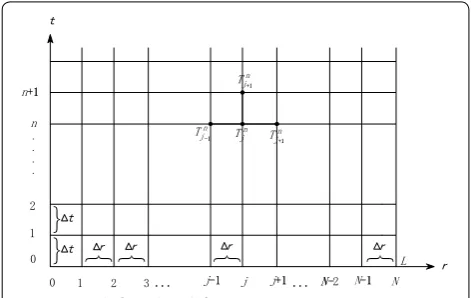
The area (r, t) is divided into the grid of step Δr, Δt, as shown in Figure 4. Then there are:
The temperature can be expressed as
Using the boundary conditions r=r1 and r=r2, respec-tively for the forward difference and backward difference gives
The terms Tn+1 0 and Tn
+1
N are determined by rearranging (2) r=j�r, j=0, 1, 2,. . .,N, L=r2−r1=N�r,
(3)
t=n�t, n=0, 1, 2, 3,. . .
(4)
T(r,t)=T(j�r,n�t)≡Tjn.
(5)
−T
n+1 1 −Tn
+1 0
r +h1T n+1 0 =f1,
(6)
T
n+1 N −Tn
+1 N−1
r +h2T
n+1 N =f2.
(7) Tn+1
0 = 1+(h11�r/)
Tn+1
1 +
f1�r
, n=0, 1, 2,. . ., j=0, $ $ $ $ % %%% D E F G (a) (b) ' G 6
U
Figure 3 Work roll cross section diagram
Q Q
M M M 1 1 1 1 7MQ
`
`
`
`
`
`
W
W U U U U
U W /
7MQ
7MQ
7MQ
Its magnitude of truncation error is Δr, and Eq. (1a) is dif-ferentially calculated to give
Which combines with Eq. (2) to give
where m= a�t
(�r)2.
Its magnitude of truncation error is (Δr)2+ (Δt), the right side of Eq. (10) includes T0n when j= 1 and TNn when
j=N − 1. These temperatures can be calculated by Eqs. (7) and (8), the superscript n+ 1 in place of n, and then the resulting T0n and TNn put into Eq. (10). The results are sum-marized as follows:
where n= 0, 1, 2,… and βi=1+ hi�r,γi = fi�r
, and i= 1 or 2.
The initial condition is
(8) TNn+1= 1+(h2�r/1 )
TNn+−11+
f2�r
,
n=0, 1, 2,. . ., j=N,
(9)
Tjn−1−2Tjn+Tjn+1
(�r)2 +
1
r
Tjn+1−Tjn−1
2�r =
1
a Tn+1
j −Tjn
�t .
(10) Tjn+1=(1− 1
2j)mTjn−1+(1−2m)Tjn+(1+21j)mTjn+1,
j=1, 2, 3,. . .,N−1, n=0, 1, 2. . .
(11) T0n+1= 1
β1(T n+1
1 +γ1), j=0,
(12a)
T1n+1=
1−2m+ m
2β1
T1n+3
2mT n
2 +
mγ1
2β1
, j=1,
(12b) Tn+1
j =
1−2j1
mTjn−1+(1−2m)Tjn+
1+2j1
mTjn+1,
j=2,. . .,N−2,
(12c) TNn+−11=
2N−3 2N−2mT
n
N−2+(1−2m+
m
β2
2N−1 2N−2)T
n
N−1
+ mγ2
β2
2N−1
2N−2, j=N−1,
(13)
TNn+1= 1
β2
TNn+1−1+γ2
, j=N,
(14)
Tj0=T(j�r)≡T(r), j=0, 1, 2,. . .,N.
Equations (11) to (14) give the finite difference expres-sion of the heat conduction equation. The solving method for this is described below.
Equation (12) provides N− 1 algebraic equations to solve the N−1 unknown nodal temperatures: Tn+1
1 , Tn
+1 2 ,. . .,Tn
+1
N−1. Due to the use of explicit form these equations are not coupled, and may be calcu-lated separately. Calculation is started with n= 0, T11, T21,. . .,TN1−1 and are determined according to Eq. (12), then the temperature values are found when
n= 1,2,…. As Tn+1 1 and Tn
+1
N−1 can be obtained by Eq. (12), then the boundary surface temperature Tn+1
0 and Tn
+1
N can be calculated respectively according to Eqs. (11) and (13).
Once a and Δr are determined, the time step Δt will be limited by the stability criterion:
3.3 Calculation of the Heat Transfer Coefficient
When the size of the hole and type of fluid are deter-mined, the heat transfer coefficient between the fluid and the inner wall is related to the temperature and velocity of the fluid. In this paper, the heat conducting fluid was L-QD330, and the initial temperature of the fluid was 300 °C. In the following section the effect of fluid velocity on heat transfer coefficient will be studied. The faster the fluid the greater the heat transfer coefficient, but the flow resistance will increase when the velocity increases, and damage to the equipment will increase. To protect the equipment and reduce pipe wear, the velocity was con-trolled within a reasonable range.
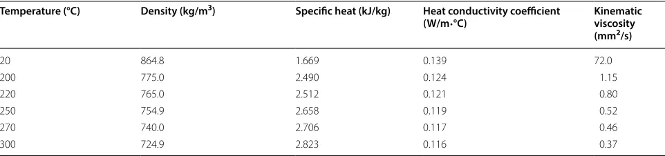
The temperature t′
f= 300 °C was used as a qualitative temperature to calculate the Reynolds number, then the calculation was checked. Table 1 describes the physical property parameters of the heat conducting fluid L-QD330.
The Reynolds number of the heat conducting fluid is Ref = umdvf , the Pr number is Prf =
cρvf
[20, 21], the Nu
number is Nuf =0.027Re0.8f Prf1/3 u
f
uw
0.25
, and when
Re > 104 the fluid flow regime is turbulent [22, 23]. There-fore, the heat transfer coefficient is h1=
Nuf
d , where
The fluid heat release per unit time is equal to the enthalpy difference of import and export, therefore, (15) m≡ a�t
(�r)2 ≤ 1 2 .
(16) h1=0.027u
0.8
mc1/3ρ1/32/3
v0.25
w v
13/60
f d0.2
Mct′
f −t
′′
f
=h1πdl
1 2
t′
f +t
′′
f
−tw
, whose
simplifi-cation is
where um is the velocity of the fluid (m/s); vf is the kine-matic viscosity of the fluid (m2/s); c is the specific heat of the fluid (kJ/kg); ρ is the density of the fluid (kg/m3); λ is the thermal conductivity of the fluid (W/m·°C); uf and uw are the fluid dynamic viscosities under fluid temperature
tf and wall temperature tw as characterization tempera-ture (Pa·s); t′′
f is the fluid export temperature when t ′ f is the qualitative temperature, and M=ρπd2
4 um is the traf-fic quality of the fluid.
The export temperature t′′
f is calculated, then input to
t′′′ f = 1 2 t′
f +t
′′
f
, so the average temperature of the fluid
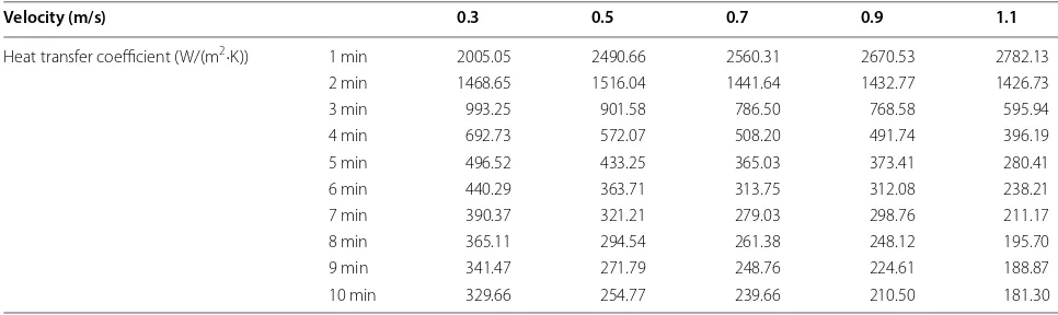
in the whole pipe can be obtained. Then this can be re-checked as a qualitative temperature, and iterated until the difference between the calculated outlet temperature and the previous outlet temperature is less than 1%. Table 2 indicates the heat transfer coefficient and average fluid temperature of the respective velocities after calculation.
The heat transfers between the roll and the outside are mainly natural convection heat transfer and thermal radi-ation in air. The natural convection heat transfer coeffi-cient of the outside is:
(17)
t′′
f =
h1πdl
tw−12t
′ f
+Mct′
f
Mc+12h1πdl
,
where tm= T+tf2
2 .
The heat transfer coefficient when the roll radiates is [18, 19]:
The heat transfer coefficient between the roll and the outside is:
Where λ, v, and Pr are the heat conductivity coefficient (W/m °C), the kinematic viscosity (W/m °C), and the
Pr number of the outside when the temperature is tm, respectively. Further, T is the average temperature of the roll (°C); σ is 5.669 × 10⁻⁸, ε is the emissivity of the roll,
and tf2 is the outside temperature (20 °C).
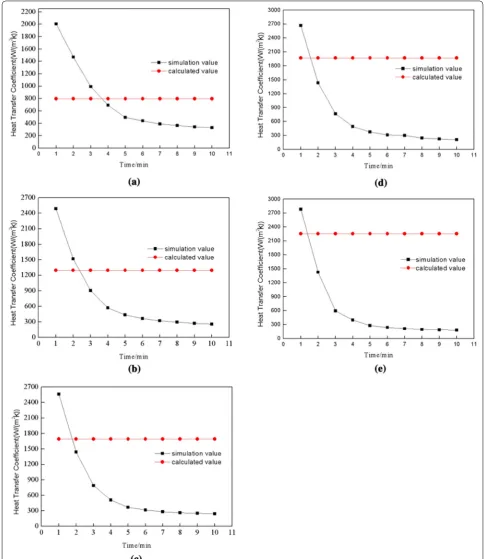
The heat transfer coefficient (h1) is calculated in the ideal circumstances of a constant wall temperature. In fact, the wall temperature gradually increased, the temperature and physical parameters of the fluid were always changing, and the heat transfer coefficient reduced. Therefore we needed to correct the calculated values. Table 3 describes the heat transfer coefficient of the respective velocities after the experiment. Calcu-lation and experimental results are shown in Figure 5. The heat transfer coefficient was corrected, and the fitting equation is shown as Eq. (20). The heat transfer coefficient has more influence than the fluid tempera-ture on the heat transfer process, so the temperatempera-ture of the fluid is the average calculating value.
Equations (11)‒(14) were programmed by C++, the
correction heat transfer coefficients h1 and h2 were generated into the equation at various velocities, and then the roll temperature was calculated under various velocities over time.
(18) h′2=0.53
gPr(T−t
f2) v2l(t
m+273)
1/4
,
(19)
h′′2=σ ε
(T +273)2+(tf2+273)2
(T +273)+(tf2+273)
h2=h′2+h′′2.
Table 1 Physical property parameters of heat conducting fluid L-QD330
Temperature (°C) Density (kg/m3) Specific heat (kJ/kg) Heat conductivity coefficient
(W/m·°C) Kinematic viscosity (mm2/s)
20 864.8 1.669 0.139 72.0
200 775.0 2.490 0.124 1.15
220 765.0 2.512 0.121 0.80
250 754.9 2.658 0.119 0.52
270 740.0 2.706 0.117 0.46
300 724.9 2.823 0.116 0.37
Table 2 Heat transfer coefficient and the average fluid temperature of the respective velocities after calculation
Velocity (m/s) 0.3 0.5 0.7 0.9 1.1
hf1 (W/(m2 K)) 597.4 1096.1 1489.4 1770.5 2055.9
4 Discussion of Numerical Simulation and Results 4.1 Numerical Simulation
Depending on the size of the roll (and the designed value of the thermostat hole), the model of the roll was built by finite element software (Pro-E), as shown in Figure 6(a). The established model was imported into Workbench for gridding, and the grid type was set to Tetra. Considering the time and accuracy of the cal-culation, it was determined that the maximum value of the grid was 5−3 mm, and the minimum value was 5−4 mm. Due to the viscosity of the heat conduction oil during the flow process, five layers of fluid bound-ary layer were set up, and the growth rate was 1.1, as shown in Figure 6(b). The heat transfer model was set as transient, the temperature unit was K, the fluid flow state was set to turbulent state, and the roll parameters were set as shown in Table 4. The initial temperature of the roll was 20 °C, and the heat transfer process of the velocity at 0.3, 0.5, 0.7, 0.9 and 1.1 m/s were numerically simulated.
(20)
h1=3009.96 exp(−t/2.54)+6.42,
h1=440.29,
t≤6 min,
t>6 min, v=0.3 m/s,
h1=4404.15 exp(−t/1.62)+114.52,
h1=433.25,
t≤5 min,
t>5 min, v=0.5 m/s,
h1=4940.27 exp(−t/1.45)+84.16,
h1=508.20,
t≤4 min,
t>4 min, v=0.7 m/s,
h1=6554.64 exp(−t/1.57)−180.69,
h1=491.74,
t≤4 min,
t>4 min, v=0.9 m/s,
h1=5784.70 exp(−t/1.49)−154.57,
h1=396.19,
t≤4 min,
t>4 min, v=1.1 m/s.
4.2 Results Analysis of Numerical Simulation
The heat transfer process under different velocities was simulated, and the temperature values of a, b, c, d and the temperature field of the roll were obtained, as shown in Figures 7, 8. This shows that the fluid heats the outside along the thermostat hole progres-sive layers. On the roll surface, four points (a, b, c, and d) were measured, and the fluid flowed through the thermostat hole successively at the four points, as shown in Figure 3(a). The temperature at point c was measured to compare with the calculated temperature. Each temperature point on the roll surface increased with time, but the rate of increase reduced. The tem-perature difference between the points did not vary with the change of time and velocity after three min-utes. The temperature difference value between import and export was approximately 30 °C. There was also a temperature difference along the axial direction of the roll. The temperature difference at the first oil hole on the roll surface (import) was bigger (up to 27 °C), and the temperature difference for the rest of the roll sur-face was small (approximately 5 °C). The nearest hole Table 3 Heat transfer coefficient of the respective velocities after the experiment
Velocity (m/s) 0.3 0.5 0.7 0.9 1.1
Heat transfer coefficient (W/(m2·K)) 1 min 2005.05 2490.66 2560.31 2670.53 2782.13
2 min 1468.65 1516.04 1441.64 1432.77 1426.73
3 min 993.25 901.58 786.50 768.58 595.94
4 min 692.73 572.07 508.20 491.74 396.19
5 min 496.52 433.25 365.03 373.41 280.41
6 min 440.29 363.71 313.75 312.08 238.21
7 min 390.37 321.21 279.03 298.76 211.17
8 min 365.11 294.54 261.38 248.12 195.70
9 min 341.47 271.79 248.76 224.61 188.87
warmed the quickest, the furthest the hole warmed the slowest, and it decreased with the reduced trend of the slope.
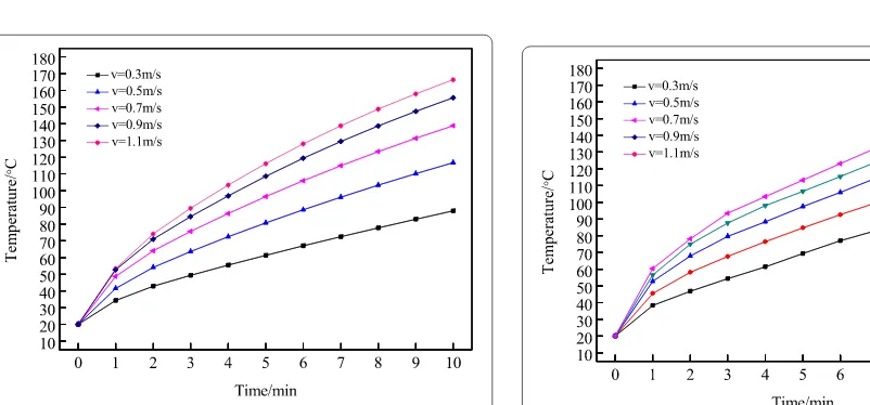
The relationship between temperature of point c and time (under different velocities) is shown in Figure 9. The greater the velocity, the faster the heat transferred, the temperature of points on the roll increased quicker, but the rate of the rise decreased.
The optimum roll temperature range was 160−250 °C for the rolling process of magnesium alloy. The time (t) and the pressure difference (ΔP) between the import and export (when the roll was heated from room tempera-ture to 200 °C under different velocities) are shown in Table 5. The trend of the change is shown in Figure 10. The fluid velocity changed from 0.3 to 1.1 m/s, t reduced from 34.4 to 15.5 minutes, the pressure increased from 0.03 to 0.32 MPa, the heating time shortened, and the velocity increased to a certain value. Further, the heat transfer increase rate decreased, but the pressure became larger and the flow resistance increased. The relation-ships between velocity (v), time (t), and the pressure dif-ference (ΔP) between the import and exports were fitted as in Eqs. (21) and (22). In the actual production, the best velocity was selected according to the required heating time, and whether different equipment could withstand the pressure.
4.3 Results Analysis of Theoretical Calculations
The roll surface temperature field (obtained by the above calculation method under different velocities with time) is shown in Figure 11. The greater the velocity is, the faster the heat transfer. The roll temperature was consist-ent with the simulation results.
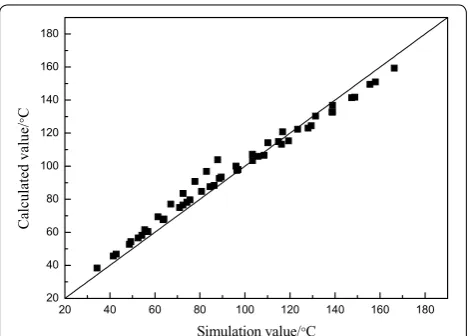
4.4 Comparative Analysis of Theoretical and Numerical Data
Calculation and simulation results of the roll tempera-ture field are compared in Figure 12. The error was 1.8%– 12.3%, which indicates the validity of the model of heat transfer theory. Temperature values of the import and export was approximately 30 °C, the difference and the influence on the magnesium alloy sheet were both bigger, therefore the fluid reverse flowed, then after a period of time it positive flowed to balance the temperature of the roll surface.
(21)
t=46.29 exp(−v/0.39)+12.65,
(22)
�P=4.01 exp(v/0.5)−4.16.
Figure 6 Three‑dimensional model diagram of the work roll
Table 4 Physical property parameters of the fluid and roll
Material Density (kg/
m3) Specific heat (kJ/
kg)
Heat conductivity coefficient (W/m·°C)
Kinematic viscosity (mm2/s)
Fluid 735 2.75 0.117 0.37
0 1 2 3 4 5 6 7 8 9 10 10
20 30 40 50 60 70 80 90 100 110 120 130 140 150
Temperature/
Time/min simulation value-a simulation value-b simulation value-c simulation value-d
(a)
0 1 2 3 4 5 6 7 8 9 10
10 20 30 40 50 60 70 80 90 100 110 120 130 140 150
Temperat
ur
e/
Time/min calculated value
simulation value-a simulation value-b simulation value-c simulation value-d
(b)
0 1 2 3 4 5 6 7 8 9 10
10 20 30 40 50 60 70 80 90 100 110 120 130 140 150 160 170 180
Temperat
ure/
Time/min
simulation value-a simulation value-b simulation value-c simulation value-d
(c)
0 1 2 3 4 5 6 7 8 9 10
20 40 60 80 100 120 140 160 180 200
Time/min
simulation value-a simulation value-b simulation value-c simulation value-d
(d)
Figure 7 Temperature simulation value of the point a, b, c, and d, and the roll temperature field (after 10 min): a v= 0.3 m/s; b v= 0.5 m/s; c
0 1 2 3 4 5 6 7 8 9 10 20
40 60 80 100 120 140 160 180 200
Time/min
simulation value-a simulation value-b simulation value-c simulation value-d
Figure 8 Temperature simulation value of the point a, b, c, and d, and the roll temperature field (after 10 min): v= 1.1 m/s
Figure 9 Simulation temperature curve of point c under different velocities
Table 5 Time and pressure values up to 200 °C
under different velocities
Velocity (m/s) 0.3 0.5 0.7 0.9 1.1
Time (min) 34.4 24.5 21.3 16.2 15.5
Pressure (MPa) 0.03 0.07 0.12 0.20 0.32
Figure 10 Time and pressure values when the roll surface temperature was heated to 200 °C under different velocities
5 Heat Transfer after Reverse Flow of Fluid
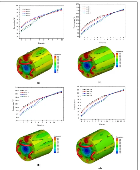
A study of the temperature required for points on the roll surface to reach equilibrium is necessary, as the required roll temperatures will vary depending on the rolling con-ditions. From the above results, when the velocity was 1.1 m/s, the heat transfer was optimum, so the process of fluid reverse flow after forward flow for different times was simulated under this velocity. The temperature of the points and the temperature field of the roll are shown in Figure 13, 14. The equilibrium time and equilibrium tem-perature (when point temtem-peratures reached the same value under different velocities) are shown in Table 6.
The results showed that the equilibrium time was substantially constant when the positive fluid flow was longer, but the equilibrium temperature increased with the velocity increase. After the reverse flow of fluid, the export temperature of the roll increased, but the length of this area range was less than 1/5 of the length of the roll, and the temperature difference (between the surface area of the hole and the surface area of non-holes) did not exceed 8 °C. The axial temperature difference at the roll import was approximately 18 °C, the high temperature zone was concentrated at 1/8 of the roll body length, and
the temperature of other positions was uniform. The sur-face temperature for the remaining 7/8 of the roll sursur-face was even more uniform. As the roll surface temperature difference was small, the rolling process could be carried out.
When the relationship between the fluid flowing time (t) and equilibrium temperature (T) is fitted we get:
Therefore we can determine the fluid flowing time according to the required roll temperature to obtain a more accurate roll temperature value.
6 Conclusions
(1) The theoretical calculation results and numerical simulation results of heat transfer between the fluid and roll were compared (the error was 1.8%‒12.3%). This showed that the heat transfer theoretical model could forecast and regulate roll temperature when magnesium alloy sheets are rolled.
(2) Compared with the traditional heating method, the method of heating the surface temperature of the roll with the fluid reduced the heating time, and the temperature distribution of the roll surface was more uniform. However, the temperature difference between import and export was bigger. The lager the velocity, the faster the heat transfer, but the rate of increase decreased.
(3) The method of fluid reverse flowing after a period of positive flowing was used to balance the tem-perature difference between import and export. The longer the time of fluid flow, the time required to reach equilibrium was constant (approximately four minutes). When the fluid forward flow time was longer, the equilibrium temperature was higher. The more accurate roll temperature can be obtained by reasonably determining the time of forward flow of fluid.
(23) T = −5400.7+5605.1 exp
−0.5(t−12.6) 70.8
2
.
1 2 3 4 5 6 7 8 9 10 20
40 60 80 100 120 140 160 180 200
Temperat
ure/
Time/min
node a node b node c node d
(a)
1 2 3 4 5 6 7 8 9 10 11 12
20 40 60 80 100 120 140 160 180 200 220
Temperature/
Time/min
node a node b node c node d
(b)
1 2 3 4 5 6 7 8 9 10 11 12 13 14 40
60 80 100 120 140 160 180 200 220 240
Temperature
/
Time/min
node a node b node c node d
(c)
1 2 3 4 5 6 7 8 9 10 11 12 13 14 15 16 40
60 80 100 120 140 160 180 200 220 240
Tempera
ture
/
Time/min
node a node b node c node d
(d)
Authors’ Contributions
J‑FZ completed the numerical simulation, data analysis and the modification of the manuscript; L‑FM guided the whole data analysis process and approved the final version; G‑HZ derived the formulas; Z‑QH, J‑BL carried out literature search and data acquisition; P‑TL reviewed and edited the manuscript. All authors read and approved the final manuscript.
Author Details
1 Heavy Machinery Engineering Research Center of the Ministry Education,
Taiyuan University of Science and Technology, Taiyuan 030024, China. 2 School
of Mechanical Engineering, Taiyuan University of Technology, Taiyuan 030024, China.
Authors’ Information
Jing‑Feng Zou, born in 1993, is a graduate candidate at Taiyuan University of Science and Technology, China. Her research interests include roller tempera‑ ture field control.
Li‑Feng Ma, born in 1977, is currently a professor at Taiyuan University of Science and Technology, China. He received his PhD degree from Taiyuan Uni-versity of Technology, China, in 2008. His research interests include magnesium alloy sheet properties study.
Guo‑Hua Zhang, born in 1991, is a graduate candidate at Taiyuan University of Science and Technology, China. Her research interests include roller tempera‑ ture field control.
Zhi‑Quan Huang, born in 1982, is currently an associate professor at
Taiyuan University of Science and Technology, China. He received his PhD degree from Taiyuan University of Science and Technology, China, in 2014. His research interests include rolling process and equipment design, light alloy deforma‑ tion process theory and technology.
Jin‑Bao Lin, born in 1979, is currently a professor at Taiyuan University of Science and Technology, China. He received his PhD degree from Shanghai Jiao Tong University, China, in 1996. His research interests include magnesium alloy plastic forming, large plastic deformation technology.
Peng‑Tao Liu, born in 1989, is currently a PhD candidate at Taiyuan Univer-sity of Technology, China. His research interests include Composite plate shape and performance.
Acknowledgements
The authors sincerely thanks to Professor Da‑Qing Fang of Xi’an Jiao Tong University for guidance on the usage of old equipment in the field, and to Professor Qing‑Xue Huang of Taiyuan University of Technology for valuable discussion.
Competing Interests
The authors declare that they no competing interests.
Funding
Supported by National Natural Science Foundation of China (Grant No. U1510131), Key Research and Development Projects of Shanxi Province of China (Grant Nos. 201603D121010, 201603D111004), Science and Technology Project of Jin Cheng City of China (Grant No. 20155010), Youth Program of National Natural Science Fund of China (Grant No. 51604181), Project of Young Scholar of Shanxi Province, Leading Talent Project of Innovative Entrepreneur‑ ial Team of Jiangsu Province (Grant No. 51501122).
Publisher’s Note
Springer Nature remains neutral with regard to jurisdictional claims in pub‑ lished maps and institutional affiliations.
Received: 5 June 2017 Accepted: 23 October 2018
References
[1] Z H Chen. Wrought magnesium alloys. Beijing: Chemical Industry Press, 2005. (in Chinese)
[2] J R Luo, Q Liu, W Liu, et al. Influence of rolling temperature on the {10̄11‑ {10̄12 twinning in rolled AZ31 magnesium alloy sheets. Acta Metallurgica Sinica, 2012, 48(6): 718‑724. (in Chinese)
[3] I A Maksoud, H Rahmed, J Rodel, et al. Investigation of the effect of strain rate and temperature on the deformability and microstructure evolution of AZ31 magnesium alloy. Mater. Sci. Eng., 2009, A504: 40‑47.
[4] H Watanabe, T Mukai, K Ishikawa. Effect of temperature of differential speed rolling on room temperature mechanical properties and texture in an AZ31 magnesium alloy. Journal of Materials Processing Tech., 2007, 182(1): 644‑647.
[5] L F M, W T Jia, J B Lin, et al. Establishment of a constitutive model of temperature‑changed rolling process for as‑cast AZ31B magnesium alloy.
Rare Metal Materials and Engineering, 2016, 45(2): 339‑345. (in Chinese)
0 1 2 3 4 5 6 7 8 9 10 11 12 13 14 15 16 17 18 20
40 60 80 100 120 140 160 180 200 220 240
Temperature
/
Time/min
node a node b node c node d
Figure 14 Temperature value of the points a, b, c, and d under different forward flow times: t = 11 min
Table 6 Equilibrium time and equilibration temperature after different flowing times
Flow time (min) 3 5 7 9 11
Equilibrium time (min) 4 4 4 4 5
[6] W T Jia, L F Ma, Z Y Ma, et al. Temperature‑changed rolling process and the flow stress of as‑cast AZ31B magnesium alloy. Rare Metal Materials and Engineering, 2016, 45(1): 152‑158. (in Chinese)
[7] W T Jia, L F Ma, Y P Jiang, et al. Mathematical temperature field model about as‑cast AZ31B magnesium alloy during hot rolling of plate. Rare Metal Materials and Engineering, 2016, 45(3): 702‑708. (in Chinese) [8] W T Jia, L F Ma, P T Liu, et al. Mathematical model of coupled thermal‑
stress about AZ31B magnesium alloy plate during hot rolling. Rare Metal Materials and Engineering, 2016, 45(5): 1175‑1181. (in Chinese) [9] Miao Q, Hu L, Wang G, et al. Fabrication of excellent mechanical proper‑
ties AZ31 magnesium alloy sheets by conventional rolling and subse‑ quent annealing. Mater. Sci. Eng., 2011, A528: 6694‑6701. (in Chinese) [10] J Z Quan, M N Duan, S J Yao, et al. China. One kind of roll preheating
device. Patent No. 201120342220.4. 2012‑05‑30.
[11] X Q Jiang, R J Cheng, F S Pan, et al. China. Roll Preheat Insulation System. Patent No. 201310467215.X. 2014‑01‑01.
[12] L F Ma, Z N Pang, Q X Huang, et al. Analysis of hot rolled cracks of casting AZ31B magnesium alloy plate. Rare Metal Materials and Engineering, 2014, 43(s1): 387‑392. (in Chinese)
[13] M J Feng, H Ji. Numerical simulation on unsteady state temperature field of high speed steel composite roll during continuous hot slab rolling.
Journal of Central South University (Science and Technology), 2012, 43(6): 2096‑2100. (in Chinese)
[14] X J Zhang. Simulation and experimental research for temperature field of work roll in 300 cold rolling mill. Yanshan University, 2010. (in Chinese) [15] P Yu. Study on temperature field of roll during cold strip. University of
Sci-ence and Technology Liaoning, 2012. (in Chinese)
[16] S X Chen, W G Li, X H Liu, et al. Thermal crown model and shifting effect analysis of work roll in hot strip mills. Journal of Iron and Steel Research, 2015, 22(9): 777‑784.
[17] W G Li, X H Liu, Z H Guo, et, al. Numerical simulation of temperature field and thermal crown of work roll during hot strip rolling. The Chinese Journal of Nonferrous Metals, 2012(11): 3176‑3184. (in Chinese)
[18] F F Kong, A R He, J Shao, et al. Finite element model for rapidly evaluating the thermal expansion of rolls in hot strip mills. Journal of University of Science and Technology Beijing, 2014(5): 674‑679. (in Chinese) [19] M J Fing, E G Wang, J C He, et al. Numerical simulation of temperature
field in high speed steel composite roll during continuous pouring process for cladding. Acta Metallurgica Sinica, 2011, 47(12): 1495‑1512. [20] C M Yu. Heat conduction. Beijing: Higher Education Press, 1983. (in
Chinese)
[21] H H Wang. Heat transfer. Chongqing: Chongqing University Press, 2006. (in Chinese)
[22] Z H Qiao. Hydromechanics. Shanxi: Shanxi Science and Technology Press, 2001. (in Chinese)