Estimation of Interchannel Time Difference in Frequency Subbands Based on Nonuniform Discrete Fourier Transform

(1)

Volume 2008, Article ID 618104,7pages doi:10.1155/2008/618104

Research Article

Estimation of Interchannel Time Difference in Frequency

Subbands Based on Nonuniform Discrete Fourier Transform

Bo Qiu, Yong Xu, Yadong Lu, and Jun Yang

Communication Acoustics Lab, Institute of Acoustics, Chinese Academy of Science, 21 Bei-Si-Huan-Xi-Lu, Beijing 100190, China

Correspondence should be addressed to Jun Yang,[email protected]

Received 5 November 2007; Accepted 23 March 2008

Recommended by Woon-Seng Gan

Binaural cue coding (BCC) is an efficient technique for spatial audio rendering by using the side information such as interchannel level difference (ICLD), interchannel time difference (ICTD), and interchannel correlation (ICC). Of the side information, the ICTD plays an important role to the auditory spatial image. However, inaccurate estimation of the ICTD may lead to the audio quality degradation. In this paper, we develop a novel ICTD estimation algorithm based on the nonuniform discrete Fourier transform (NDFT) and integrate it with the BCC approach to improve the decoded auditory image. Furthermore, a new subjective assessment method is proposed for the evaluation of auditory image widths of decoded signals. The test results demonstrate that the NDFT-based scheme can achieve much wider and more externalized auditory image than the existing BCC scheme based on the discrete Fourier transform (DFT). It is found that the present technique, regardless of the image width, does not deteriorate the sound quality at the decoder compared to the traditional scheme without ICTD estimation.

Copyright © 2008 Bo Qiu et al. This is an open access article distributed under the Creative Commons Attribution License, which permits unrestricted use, distribution, and reproduction in any medium, provided the original work is properly cited.

1. INTRODUCTION

Since 1990, joint stereo coding algorithm has been widely used in the two-channel audio coding. Various techniques have been developed for compressing stereo or multichannel audio signals. Recently, the ISO/MPEG standardization group has published a new audio standard, that is, MPEG Surround, which is a feature-rich open standard compres-sion technique for multichannel audio signals [1]. MPEG Surround coding can be regarded as an enhancement of the joint stereo coding and an extension of BCC [2–5]. BCC exploits binaural cue parameters for capturing the spatial image of multichannel audio and enables low-bit-rate transmission by transmitting mono signals plus side information in relation to binaural perception.

BCC is based on the spatial hearing theory [6], which uses the binaural cues such as interaural level diﬀerence (ILD), interaural time diﬀerence (ITD), and interaural coherence (IC) for rendering spatial audio. For multichannel audio signals, the corresponding spatial cues contained in signals, disregarding playback scenarios, are ICLD, ICTD,

and ICC. Generic BCC scheme is illustrated in Figure 1. As input multichannel audio signals are downmixed into mono sum signal, side information which comprises some interchannel cues is also analyzed and obtained, and then both sum signal and side information are transmitted to the decoder. Finally, these cues are generated from the side information, and based on them BCC, synthesis generates the output multichannel audio signals. The detailed system implementation and variations of BCC are presented in [7].

(2)

Input

Coder Decoder Output

Downmix

Sum signal

Synthesis

Side information Cues

estimation

Figure1: Generic scheme of BCC.

spatial image width could be widened significantly and a better overall quality could be achieved compared to the BCC scheme without using the time diﬀerence cue.

Generic BCC scheme estimates ICTD in frequency sub-bands partitioned according to psychoacoustic critical sub-bands [9]. When DFT is used to implement time-to-frequency transform, the subband bandwidth in the range of low frequency is much narrower than that in the high frequency range due to the uniform sampling. However, to account for human auditory perception, spatial cues contained in low-frequency subbands are more important than those in high-frequency subbands. The DFT method may not analyze subband properties properly so that the BCC scheme with the ICTD estimation is unable to improve the audio quality and even deteriorates it.

An alternative solution is to employ the nonuniform discrete Fourier transform (NDFT). The advantage of the NDFT is that localization of frequency bins can be adjusted as requested. In this paper, we propose a novel NDFT-based method to estimate ICTD more accurately than in the DFT-based solutions. Firstly, a subband factor is calculated to evaluate the coherence degree of two channels and then decide whether it is necessary to estimate ICTD. A new subjective testing is designed to assess the proposed BCC scheme from many references to [8] and results are in accordance with expectations. The rest of this paper is organized as follows. Section 2 introduces the concept of NDFT.Section 3discusses ICTD estimation based on DFT. Section 4 presents the improved ICTD estimation. Subjective tests are described inSection 5. Finally, a brief conclusion is drawn inSection 6.

2. CONCEPT OF NDFT

2.1. Introduction

Traditional DFT is obtained by sampling the continuous frequency domain at N points evenly spaced around the unit circle in thez-plane. Therefore, if the temporal sample rate andN are fixed, all the frequency points are uniformly distributed from zero to the temporal sample rate. From the point of view of the human auditory perception, the main drawback of this approach is the use of an equally spaced

k2

k4 k0

k3 k1

k5

(a) DFT

k2

k4 k0

k3

k1

k5

k7

k6

(b) NDFT

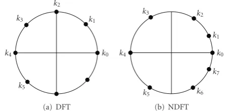
Figure2: Comparison of the sampling methods between DFT and NDFT.

frequency range which leads into a transform of the whole frequency spectrum for the sampling rate as a constraint.

Diﬀerent from the uniform DFT, NDFT enables the anal-ysis of arbitrary frequency ranges with irregular intervals.N frequency points of NDFT are nonuniformly spaced around the unit circle in the z-plane. By choosing the frequency points appropriately, NDFT can change the distribution of frequency points in diﬀerent subbands. It is possible to increase the frequency points in low-frequency bands and accordingly decrease those in high-frequency bands. Improved frequency accuracy may be helpful for spatial hearing.

2.2. Definition of NDFT

The nonuniform discrete Fourier transform pair is defined as follows [10]:

Fkm

= N−1

n=0

f(n)e−jkmn_,

f(n)= 1

M

M−1

m=0 Fkm

ejkmn_,

(1)

whereMandNare the number of frequency sampling points and temporal sampling points, respectively.km may be any

real number between 0 and 2π. It is known that the diﬀerence between DFT and NDFT is mostly the manner of frequency sampling, that is, the selection ofkm.

Figure 2shows the sample locations obtained by DFT and NDFT in z-plane as M is 8. For the equal interval sampling of DFT,kmis given by

km= 2π

8×m, m=0, 1, 2,. . ., 7. (2)

For the nonuniform interval sampling,kmcan be selected as

follows,

km= 2π

12×m, m=0, 1, 2, 4, 6, 8, 10, 11. (3)

(3)

For the z-transform in the unit circle, z = ejw_. _One

dimensional NDFT of a sequencex(n) with a length ofNis defined as [11]

Xzk

= N−1

n=0

x(n)z−kn, k=0, 1,. . .,N−1, (4)

where z1,z2,. . .,zN−1 are N distinct points nonuniformly spaced around the unit circle in thez-plane. The matrix form of NDFT is

X=Dx, (5)

where X= ⎡ ⎢ ⎢ ⎢ ⎢ ⎢ ⎢ ⎣

Xz0 Xz1 .. . XzN−1

⎤ ⎥ ⎥ ⎥ ⎥ ⎥ ⎥ ⎦

, x=

⎡ ⎢ ⎢ ⎢ ⎢ ⎢ ⎣ x(0) x(1) .. . x(N−1)

⎤ ⎥ ⎥ ⎥ ⎥ ⎥ ⎦, D= ⎡ ⎢ ⎢ ⎢ ⎢ ⎢ ⎢ ⎣

1 z−1

0 z−02 · · · z−

(N−1)

0

1 z−11 z−12 · · · z−(

N−1) 1 ..

. ... ... . .. ...

1 z−N1−1 zN−−21 · · · z−N(−N1−1)

⎤ ⎥ ⎥ ⎥ ⎥ ⎥ ⎥ ⎦ . (6)

The matrixDis a Vandermonde matrix and determined by the choice of theNpointszk. As theNpointszkare not the

same, the determinant ofDis not zero. Therefore, the inverse NDFT exists and is unique, andxcan be calculated byx =

D−1_X.

3. ICTD ESTIMATION

3.1. Time-to-frequency transform

Because of the requirement of real-time data, audio signals are processed frame by frame. Traditional BCC scheme implements time-to-frequency transform via DFT (FFT). The analysis window is depicted inFigure 3. The solid line represents the Hanning window for the current frame. The zero-padding parts to each side are not given in the figure. The dashed lines show parts of Hanning windows for the previous two frames and the next two ones. Each frame containsWtemporal data which is windowed by a Hanning window with a length of W. Zzeros are padded to each side and the overall length is W+ 2Z.There are 50% overlapping between adjacent frames. This means that the first half of the data of the current frame is overlapped with the second half of the data of the previous frame. Actually, it is shown in Figure 3 that all the temporal data are windowed by a weight of a constant value 1. Therefore, there is no need to add a synthesis window in the decoding end. Perfect reconstruction can be achieved without a synthesis window.

In our schemes, the value ofWis 896 and the value ofZ is 64. Thus, a 1024-point DFT is carried out to get frequency data. It should be noted that all signals selected have the same sampling rate of 44.1 kHz.

W/2 W/2 1 0 Z Z W indo w

Time index (n) Figure3: Analysis window.

After time-to-frequency transform, two-channel signals are downmixed into mono sum signal. Meanwhile, BCC cues are estimated in frequency subbands. According to the spatial hearing theory, a nonuniform partition of subbands is chosen. As the spectrum is symmetric, only the firstN/2 + 1 (513 for 1024-point DFT) spectral bins are divided into subbands. In this paper, we use 27 subbands to approximate the psychoacoustic critical bands.Table 1shows the number of spectral bins and the index of the first spectral bins in each subband.

3.2. ICTD estimation

Suppose thatτmax is the maximum absolute value of ICTD, phase wrapping will not occur in subbands at frequencies below 1/2τmaxHz. The slope of the phase diﬀerence in these subbands between left and right channels is given by

Φ(i)=argX1(i)X2∗(i)

, (7)

whereX1(i) andX2(i) are denoted as spectral coeﬃcients in current subband of left and right channels, respectively, and iis the spectral index. Without phase wrapping, we have

∧

Φ(i)=a1i, (8)

where Φ∧(i) is the predicted value of the phase diﬀerence. Hence,

a1=Φ∧(i+ 1)−Φ∧(i), (9)

and ICTD can be obtained from the slopea1by using

ICTD(b)= a1N

2πFs, (10)

whereFsis the sampling rate. When phase wrapping occurs

above 1/2τmaxHz, unwrappingΦ∧ (i) is required. The group delay is then estimated as before. The predicted phase diﬀerence is

∧

Φ(i)=a1i+a0. (11)

(4)

Table1: Partition of subbands for DFT.

(a) Number of spectral bins in each subband

Subbands B1 B2 B3 B4 B5 B6 B7 B8 B9

Bins number 2 2 2 2 2 2 2 2 4

Bins number 4 4 4 4 6 6 8 8 12

Bins number 16 16 20 28 36 64 64 80 112

(b) Index of the first spectral bin in each subband

Index 0 2 4 6 8 10 12 14 16

Index 20 24 28 32 36 42 48 56 64

Index 76 92 108 128 156 192 256 320 400

4. NDFT-BASED ICTD ESTIMATION

From Table 1 in Section 3, it is noted that the number of spectral bins diﬀers greatly between subbands. There are more spectral bins in high-frequency subbands than those in low frequency subbands. Thus, the estimated ICTD in low-frequency subbands may not be correct because of few spectral bins obtained. Moreover, when left and right channels are not fully coherent, that is, no time diﬀerence between the two channels, the ICTD may be estimated as a nonzero value. Here, an NDFT-based method is proposed to improve the ICTD estimation.

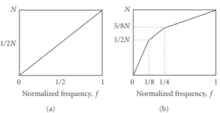
Given the frequency width is 1 and the number of spectral bins is N, uniform DFT mapping is shown in

Figure 4(a). For NDFT method, proper km are chosen to

realize the nonuniform mapping from frequency width to the number of spectral bins. On the one hand, the bins in low-frequency subbands are increased by 2 times. On the other hand, they are appropriately decreased by half in high-frequency subbands. Meanwhile, they are unchanged in middle frequency subbands as depicted in Figure 4(b). This means that the number of the selectedkm is fourfold

between 0 and 1/16π while unchanged between 1/16π and 1/8π. In order to keep the same overall number of sampling points with the DFT-based scheme, the number of km is

correspondingly reduced by half between 1/8π and 1/2π. Above 1/2π in the unit circle,km are selected symmetrically

to the first half part.

For the convenience of comparison, our NDFT-based scheme is also based on a 1024-point transform. In the NDFT method, spectral bins are also partitioned into 27 subbands as shown in Table 2(a). Obviously, the number of spectral bins in each subband is diﬀerent from the DFT scheme. Correspondingly, the index of the first spectral bin in each subband is given inTable 2(b).

Comparing Tables1(a) and2(a), the number of spectral bins has been adjusted to reduce the imbalance between

1/2N N

0 1/2 1

Normalized frequency,f (a)

N

5/8N 1/2N

0 1/8 1/4 1

Normalized frequency,f (b)

Figure4: Comparison of mapping between DFT and NDFT: (a) DFT mapping, (b) NDFT mapping.

subbands. Similar to the DFT-based method described in

Section 3.2, the phase diﬀerence between left and right channels can be calculated by

a1=Φ∧(i)−Φ∧(i−1)×σ, (12)

whereσis chosen as 1/4 in low-frequency bands, 1 in middle frequency bands and 2 in high-frequency bands, respectively. Then we can estimate the ICTD in each subband using (10). In the case that the two channels are not coherent, that is, with no time diﬀerence, it is not necessary to estimate ICTD. A subband coherence factorαis used to determine whether or not estimate the ICTD, which is calculated by

α= X1(i)X2∗(i)

_X1₍_i₎_X∗

1(i)

1/2

X2(i)X2∗(i)

1/2. (13)

(5)

Table2: Partition of bins for NDFT.

(a) Number of spectral bins in each subband

Bins number 8 8 8 8 8 8 8 8 16

Bins number 16 16 16 16 24 24 32 32 12

Bins number 16 16 20 14 18 32 32 40 56

(b) Index of the first spectral bin in each subband

Index 0 8 16 24 32 40 48 56 64

Index 80 96 112 128 144 168 192 224 256

Index 268 284 300 320 334 352 384 416 456

5. SUBJECTIVE TEST

5.1. Test design

Subjective tests are conducted using the guideline by ITU-R 1116 and ITU-ITU-R 1534 [11, 12]. There are 12 persons (including 3 females and 9 males, who are all volunteers in our group) participating as subjects in the test. Being trained, most of them are experienced listeners. The playback we used is TAKSTAR TS-610 headphone connected to an external sound card (Creative 24-bit Sound Blaster Live).

Eight diﬀerent kinds of 2-channel stereo audio excerpts are selected as the test material. All of them present a wide auditory image, and most of them are binaural or 3D audio. If the auditory images are changed, it is easy for subjects to perceive. Each excerpt is processed in 4 diﬀerent ways containing the reference audio which keeps unchanged as follows:

case A: reference, it is the same with the original excerpt but hidden in the test;

case B: DFT-based ICTD estimation, the BCC analysis and synthesis with ICLD, ICC, and DFT-based ICTD;

case C: NDFT-based ICTD estimation, the BCC analysis and synthesis with ICLD, ICC, and NDFT-based ICTD;

case D: without ICTD, the BCC analysis and synthesis only with ICLD and ICC.

Each subject should grade excerpts in two aspects. On the one hand, it needs to estimate reconstructed image width of audio signals synthesized by BCC. On the other hand, subjects should assess the overall audio quality. The image width and the overall quality are both measured by 5 scales. The scales for overall quality are shown in Table 3. Scores are given by subjects completely according to their personal perception.

Table3: Grades and scales.

Grade Overall quality

5 No diﬀerence

4 Slight diﬀerence not annoying

3 Slightly annoying

2 Annoying

1 Very annoying

Figure5: MatLab user interface for width evaluation.

5.2. Image width evaluation

(6)

coordinates of an auditory event. 0 is the perceptual position nearest to the left ear and 10 nearest to the right ear. Subjects are required to listen to the reference and choose one of the auditory events at a time when they sound mostly deviated from the central position then give the coordinate value in a scale of 5. Next, subjects should listen to the other 3 excerpts and give coordinate value of the same auditory events at that time contained in these excerpts. Assuming the value for reference excerpt isa, and that for one processed excerpt isb, the subjective score for image width can be calculated by

u=|_|b−5|

a−5|×5, (14)

where u is valued within the range from 0 to 5. As the reference has the widest auditory image, the value of a is not 5, and|b−5|is always less than|a−5|. Moreover, as the corresponding auditory events are chosen at the same temporal point, the left and right channels would not be interchanged, which is confirmed in our tests. The use of (14) makes it convenient for image width assessment as well as the audio quality evaluation.

5.3. Results and discussions

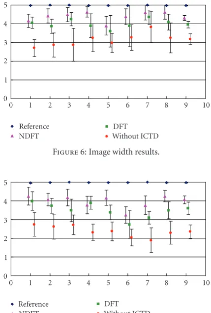
Subjective test results for the evaluation of image width and overall quality are shown in Figures 6 and 7, respectively. Both the corresponding means and 95% confidence intervals are marked.

It can be seen from Figure 6 that the scheme without ICTD results in a worst auditory image for all excerpts with lowest scores, because the synthesizing process compresses the image width of original signals. The auditory image widths of excerpts are diﬃcult for subjects to perceive due to the wider 95% confidence interval. Obviously, the scores of the NDFT-based scheme are the highest in the three processed schemes. These excerpts are most approximate to original signals with a wider auditory image rather than the other two kinds of excerpts. It means that NDFT-based ICTD estimation is more accurate than the DFT-based one as expected. The average scores in the four cases are depicted in the right part ofFigure 6, where the value “9” in the abscissa represents “average.” The average score for the case B, C, and D is 4.3, 3.9, and 3.2, respectively. It validates that the NDFT-based scheme is superior to the DFT-NDFT-based scheme.

Results for the overall quality evaluation are shown in

Figure 7. Generally, the schemes without ICTD may have the best audio quality disregarding image width. But it may change auditory image, and the decoded audio will not gain an ambient image, which aﬀects the perception quality more or less and lead to a significant diﬀerence to original audios. Therefore ICTD estimation should be adopted in BCC schemes for improving the overall quality considering image width. It is clear fromFigure 7that the scheme without ICTD has the lowest scores and the average value is 2.3, whereas the BCC scheme with DFT-based or NDFT-based ICTD estimation has an advantage over it. Moreover, the NDFT-based scheme yields higher scores than the DFT based scheme except for the excerpt sample 4. It is from the

0 1 2 3 4 5

0 1 2 3 4 5 6 7 8 9 10

Reference DFT

NDFT Without ICTD

Figure6: Image width results.

0 1 2 3 4 5

0 1 2 3 4 5 6 7 8 9 10

Reference DFT

NDFT Without ICTD

Figure7: Overall quality results.

right part of Figure 7 that the average score for the DFT-based scheme and NDFT-DFT-based scheme are 3.6 and 4.1, respectively. Obviously, NDFT-based scheme is better than the DFT-based scheme, and it is the best choice in terms of the audio quality and image width.

6. CONCLUSION

This paper presents a novel algorithm to estimate the inter-channel time diﬀerence by using the nonuniform discrete Fourier transform. The frequency bins can be adjusted as requested by integrating this algorithm with the binaural cue coding approach. Consequently, the decoded audio image width is improved compared to the traditional DFT-based method. On the other hand, the sound quality is not deteriorated by adding this algorithm module in the BCC scheme.

A subjective testing was designed and implemented. The evaluation result proves that this NDFT-based ICTD scheme is the optimal choice in terms of the audio image width and the audio quality.

ACKNOWLEDGMENT

(7)

REFERENCES

[1] http://www.mpegsurround.com/.

[2] J. Herre, “From joint stereo to spatial audio coding—recent progress and standardization,” in Proceedings of the 7th International Conference on Digital Audio Eﬀects (DAFx ’04), pp. 157–162, Naples, Italy, October 2004.

[3] C. Faller and F. Baumgarte, “Eﬃcient representation of spatial audio using perceptual parametrization,” inProceedings of the IEEE Workshop on Applications of Signal Processing to Audio and Acoustics (WASPAA ’01), pp. 199–202, New Paltz, NY, USA, October 2001.

[4] C. Faller and F. Baumgarte, “Binaural cue coding—part II: schemes and applications,”IEEE Transactions on Speech and Audio Processing, vol. 11, no. 6, pp. 520–531, 2003.

[5] C. Faller, “Coding of MPEG Surround compatible with diﬀ er-ent playback formats,” inProceedings of the 117th Convention of the Audio Engineering Society (AES ’04), San Francisco, Calif, USA, October 2004.

[6] J. P. Blauert,Spatial Hearing, MIT Press, Cambridge, Mass, USA, 1997.

[7] C. Faller, “Parametric coding of spatial audio,” Ph.D. thesis, Ecole Polytechnique F´ed´erale de Lausanne, Lausanne, Switzer-land, July 2004.

[8] C. Tournery and C. Faller, “Improved time delay analysis /synthesis for parametric stereo audio coding,” inProceedings of the 120th Convention of the Audio Engineering Society (AES ’06), Paris, France, May 2006.

[9] B. C. J. Moore,An Introduction to the Psychology of Hearing, Academic Press, London, UK, 5th edition, 2003.

[10] S. Bagchi and S. K. Mitra,The Nonuniform Discrete Fourier Transform and Its Applications in Signal Processing, Kluwer Academic Publishers, Boston, Mass, USA, 1999.

[11] Rec. ITU-R BS.1116-1, “Methods for the subjective assessment of small impairments in audio systems including multi-channel sound systems,” ITU, 1997.